Pre-requisites

You should know what a Bayes Factor is and what a p value is.

Overview

Sellke et al (Thomas Sellke 2001) study the following question (paraphrased and shortened here).

Consider the situation in which experimental drugs D1; D2; D3; etc are to be tested. Each test will be thought of as completely independent; we simply have a series of tests so that we can explore the frequentist properties of p values. In each test, the following hypotheses are to be tested: $$H_0 : D_i \text{ has negligible effect}$$ versus $$H_1 : D_i \text{ has a non-negligible effect}.$$

Suppose that one of these tests results in a p value $\approx p$. The question we consider is: How strong is the evidence that the drug in question has a non-negligible effect?

The answer to this question has to depend on the distribution of effects under $H_1$. However, Sellke et al derive a bound for the Bayes Factor. Specifically they show that, provided $p<1/e$, the BF in favor of $H_1$ is not larger than $$1/B(p) = -[e p \log(p)]^{-1}.$$ (Note: the inverse comes from the fact that here we consider the BF in favor of $H_1$, whereas Sellke et al consider the BF in favor of H_0).

Here we illustrate this result using Bayes Theorem to do calculations under a simple scenario.

Details

Let $\theta_i$ denote the effect of drug $D_i$. We will translate the null $H_0$ above to mean $\theta_i=0$. We will also make an assumption that the effects of the non-null drugs are normally distributed $N(0,\sigma^2)$, where the value of $\sigma$ determines how different the typical effect is from 0.

Thus we have: $$H_{0i}: \theta_i = 0$$ $$H_{1i}: \theta_i \sim N(0,\sigma^2)$$ .

In addition we will assume that we have data (e.g. the results of a drug trial) that give us imperfect information about $\theta$. Specifically we assume $X_i | \theta_i \sim N(\theta_i,1)$. This implies that: $$X_i | H_{0i} \sim N(0,1)$$ $$X_i | H_{1i} \sim N(0,1+\sigma^2)$$

Consequently the Bayes Factor (BF) comparing $H_1$ vs $H_0$ can be computed as follows:

BF= function(x,s){dnorm(x,0,sqrt(s^2+1))/dnorm(x,0,1)}

Of course the BF depends both on the data $x$ and the choice of $\sigma$ (here s in the code).

We can plot this BF for $x=1.96$ (which is the value for which $p=0.05$):

s = seq(0,10,length=100)
plot(s,BF(1.96,s),xlab="sigma",ylab="BF at p=0.05",type="l",ylim=c(0,4))
BFbound=function(p){1/(-exp(1)*p*log(p))}
abline(h=BFbound(0.05),col=2)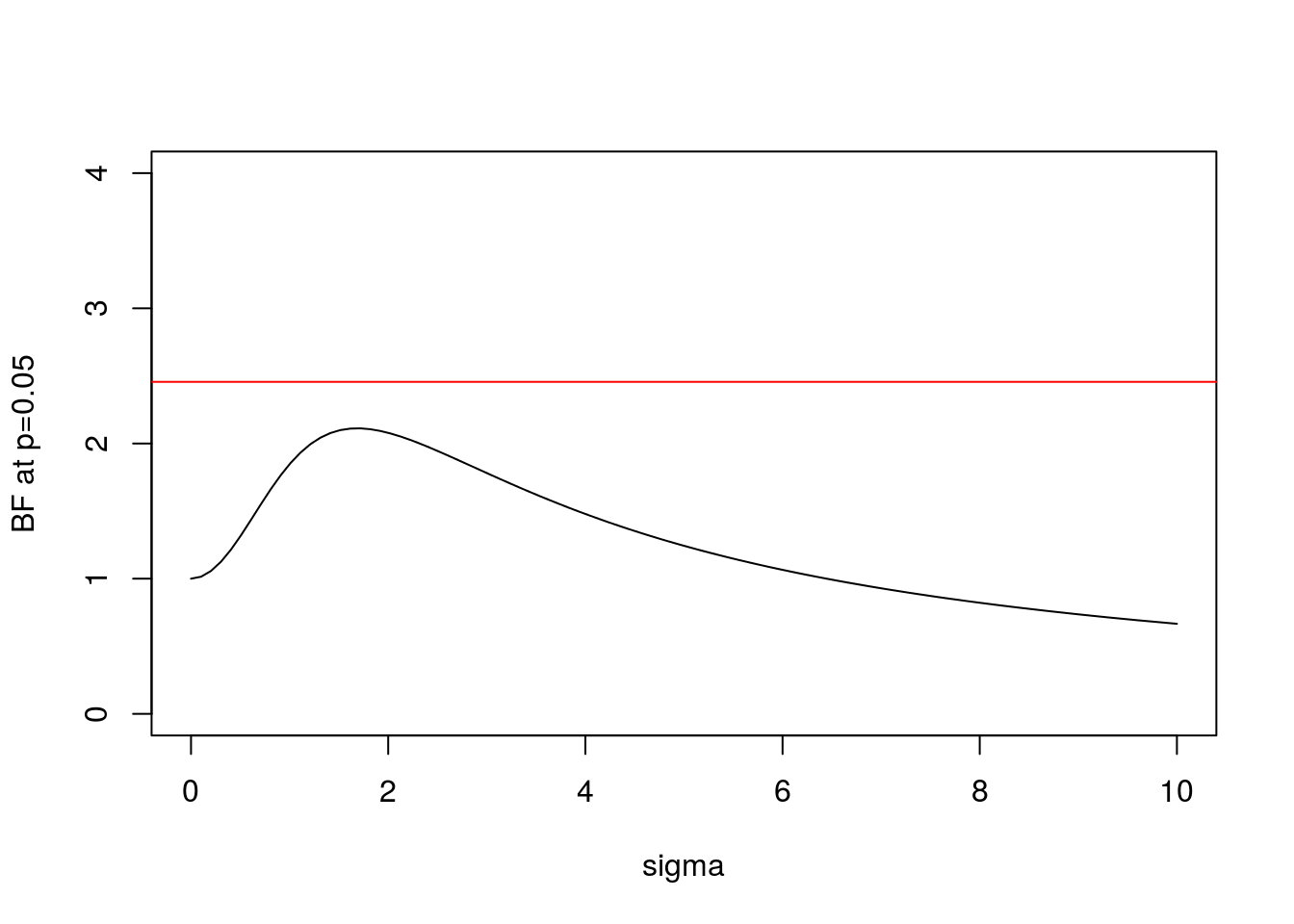

Here the horizontal line shows the bound on the Bayes Factor computed by Sellke et al.

And here is the same plot for $x=2.58$ ($p=0.01$):

plot(s,BF(2.58,s),xlab="sigma",ylab="BF at p=0.01",type="l",ylim=c(0,10))
abline(h=BFbound(0.01),col=2)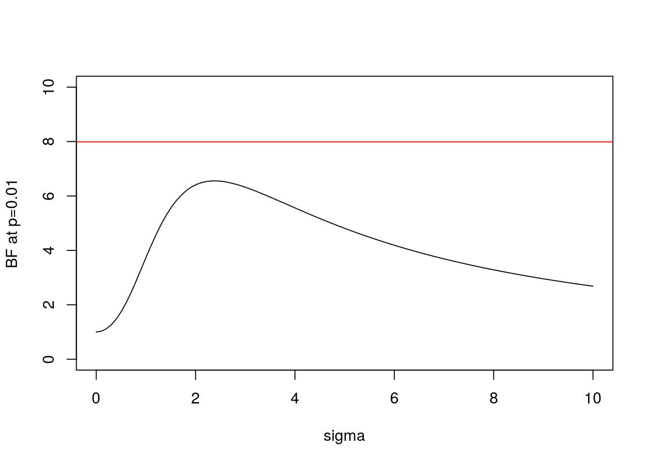

Note some key features:

• In both cases the BF is below the bound given by Sellke et al, as expected.
• As $\sigma$ increases from 0 the BF is initially 1, rises to a maximum, and then gradually decays. This behavior, which occurs for any $x$, perhaps helps provide intuition into why it is even possible to derive an upper bound.
• In the limit as $\sigma \rightarrow \infty$ it is easy to show that (for any $x$) the BF $\rightarrow 0$. This is an example of “Bartlett’s paradox”, and illustrates why you should not just use a “very flat” prior for $\theta$ under $H_1$: the Bayes Factor will depend on how flat you mean by “very flat”, and in the limit will always favor $H_0$.

sessionInfo()

R version 3.3.0 (2016-05-03)
Platform: x86_64-apple-darwin13.4.0 (64-bit)
Running under: OS X 10.10.5 (Yosemite)

locale:
[1] en_NZ.UTF-8/en_NZ.UTF-8/en_NZ.UTF-8/C/en_NZ.UTF-8/en_NZ.UTF-8

attached base packages:
[1] stats     graphics  grDevices utils     datasets  methods   base     

other attached packages:
 [1] tidyr_0.4.1     dplyr_0.5.0     ggplot2_2.1.0   knitr_1.15.1   
 [5] MASS_7.3-45     expm_0.999-0    Matrix_1.2-6    viridis_0.3.4  
 [9] workflowr_0.3.0 rmarkdown_1.3  

loaded via a namespace (and not attached):
 [1] Rcpp_0.12.5      git2r_0.18.0     plyr_1.8.4       tools_3.3.0     
 [5] digest_0.6.9     evaluate_0.10    tibble_1.1       gtable_0.2.0    
 [9] lattice_0.20-33  shiny_0.13.2     DBI_0.4-1        yaml_2.1.14     
[13] gridExtra_2.2.1  stringr_1.2.0    gtools_3.5.0     rprojroot_1.2   
[17] grid_3.3.0       R6_2.1.2         reshape2_1.4.1   magrittr_1.5    
[21] backports_1.0.5  scales_0.4.0     htmltools_0.3.5  assertthat_0.1  
[25] mime_0.5         colorspace_1.2-6 xtable_1.8-2     httpuv_1.3.3    
[29] labeling_0.3     stringi_1.1.2    munsell_0.4.3