Pre-requisites

• Likelihood Ratio.

Example

Suppose that we are considering whether to model some data \(X\) as normal or log-normal. In this case we’ll assume the truth is that the data are log normal, which we can simulate as follows:

X = exp(rnorm(1000,-5,2))

We will use \(Z\) to denote \(\log(X)\):

Z = log(X)

And let’s check by graphing which looks more normal:

par(mfcol=c(2,2))
hist(X)
hist(Z)
qqnorm(X)
qqnorm(Z)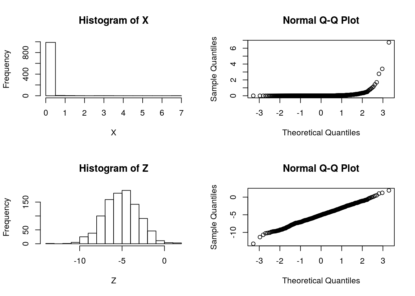

So it is pretty clear that the model ``\(M_2: \log(X)\) is normal" is better than the model “\(M_1: X\) is normal”.

Now consider computing a “log-likelihood” for each model.

To compute a log-likelihood under the model “X is normal” we need to also specify a mean and variance (or standard deviation). We use the sample mean and variance here:

sum(dnorm(X, mean=mean(X), sd=sd(X),log=TRUE))

[1] -135.3375

Doing the same for \(Z\) we obtain:

sum(dnorm(Z, mean=mean(Z), sd=sd(Z),log=TRUE))

[1] -2125.232

Done this way the log-likelihood for \(M_1\) appears much larger than the log-likelihood for \(M_2\), contradicting both the graphical evidence and the way the data were simulated.

The right way

The explanation here is that it does not make sense to compare a likelihood for \(Z\) with a likelihood for \(X\) because even though \(Z\) and \(X\) are 1-1 mappings of one another (\(Z\) is determined by \(X\), and vice versa), they are formally not the same data. That is, it does not make sense to compute \[\text{"LLR"} := \log(p(X|M_1)/p(Z|M_2))\].

However, we could compute a log-likelihood ratio for this problem as \[\text{LLR} := log(p(X|M_1)/p(X|M_2)).\] Here we are using the fact that the model \(M_2\) for \(Z\) actually implies a model for \(X\): \(Z\) is normal if and only if \(X\) is log-normal. So a sensible LLR would be given by:

sum(dnorm(X, mean=mean(X), sd=sd(X),log=TRUE)) - sum(dlnorm(X, meanlog=mean(Z), sdlog=sd(Z),log=TRUE))

[1] -3080.778

The fact that the LLR is very negative supports the graphical evidence that \(M_2\) is a much better fitting model (and indeed, as we know – since we simulated the data – \(M_2\) is the true model).

sessionInfo()

R version 3.3.0 (2016-05-03)
Platform: x86_64-apple-darwin13.4.0 (64-bit)
Running under: OS X 10.10.5 (Yosemite)

locale:
[1] en_NZ.UTF-8/en_NZ.UTF-8/en_NZ.UTF-8/C/en_NZ.UTF-8/en_NZ.UTF-8

attached base packages:
[1] stats     graphics  grDevices utils     datasets  methods   base     

other attached packages:
 [1] tidyr_0.4.1     dplyr_0.5.0     ggplot2_2.1.0   knitr_1.15.1   
 [5] MASS_7.3-45     expm_0.999-0    Matrix_1.2-6    viridis_0.3.4  
 [9] workflowr_0.3.0 rmarkdown_1.3  

loaded via a namespace (and not attached):
 [1] Rcpp_0.12.5      git2r_0.18.0     plyr_1.8.4       tools_3.3.0     
 [5] digest_0.6.9     evaluate_0.10    tibble_1.1       gtable_0.2.0    
 [9] lattice_0.20-33  shiny_0.13.2     DBI_0.4-1        yaml_2.1.14     
[13] gridExtra_2.2.1  stringr_1.2.0    gtools_3.5.0     rprojroot_1.2   
[17] grid_3.3.0       R6_2.1.2         reshape2_1.4.1   magrittr_1.5    
[21] backports_1.0.5  scales_0.4.0     htmltools_0.3.5  assertthat_0.1  
[25] mime_0.5         colorspace_1.2-6 xtable_1.8-2     httpuv_1.3.3    
[29] labeling_0.3     stringi_1.1.2    munsell_0.4.3