Last updated: 2026-07-29

Checks: 6 1

Knit directory: misc/analysis/

This reproducible R Markdown analysis was created with workflowr (version 1.7.2). The Checks tab describes the reproducibility checks that were applied when the results were created. The Past versions tab lists the development history.


The R Markdown file has staged changes. To know which version of the R Markdown file created these results, you’ll want to first commit it to the Git repo. If you’re still working on the analysis, you can ignore this warning. When you’re finished, you can run wflow_publish to commit the R Markdown file and build the HTML.

Great job! The global environment was empty. Objects defined in the global environment can affect the analysis in your R Markdown file in unknown ways. For reproduciblity it’s best to always run the code in an empty environment.

The command set.seed(1) was run prior to running the code in the R Markdown file. Setting a seed ensures that any results that rely on randomness, e.g. subsampling or permutations, are reproducible.

Great job! Recording the operating system, R version, and package versions is critical for reproducibility.

Nice! There were no cached chunks for this analysis, so you can be confident that you successfully produced the results during this run.

Great job! Using relative paths to the files within your workflowr project makes it easier to run your code on other machines.

Great! You are using Git for version control. Tracking code development and connecting the code version to the results is critical for reproducibility.

The results in this page were generated with repository version a2769cb. See the Past versions tab to see a history of the changes made to the R Markdown and HTML files.

Note that you need to be careful to ensure that all relevant files for the analysis have been committed to Git prior to generating the results (you can use wflow_publish or wflow_git_commit). workflowr only checks the R Markdown file, but you know if there are other scripts or data files that it depends on. Below is the status of the Git repository when the results were generated:


Ignored files:
    Ignored:    .DS_Store
    Ignored:    .Rhistory
    Ignored:    .Rproj.user/
    Ignored:    .claude/
    Ignored:    GSE87571/
    Ignored:    analysis/.RData
    Ignored:    analysis/.Rhistory
    Ignored:    analysis/ALStruct_cache/
    Ignored:    analysis/ebproj_01.html
    Ignored:    data/.Rhistory
    Ignored:    data/methylation-data-for-matthew.rds
    Ignored:    data/pbmc/
    Ignored:    data/pbmc_purified.RData

Untracked files:
    Untracked:  .dropbox
    Untracked:  GSE41037/
    Untracked:  Icon
    Untracked:  Rplots.pdf
    Untracked:  analysis/GHstan.Rmd
    Untracked:  analysis/GTEX-cogaps.Rmd
    Untracked:  analysis/PACS.Rmd
    Untracked:  analysis/Rplot.png
    Untracked:  analysis/SPCAvRP.rmd
    Untracked:  analysis/abf_comparisons.Rmd
    Untracked:  analysis/admm_02.Rmd
    Untracked:  analysis/admm_03.Rmd
    Untracked:  analysis/bispca.Rmd
    Untracked:  analysis/cache/
    Untracked:  analysis/cholesky.Rmd
    Untracked:  analysis/compare-transformed-models.Rmd
    Untracked:  analysis/cormotif.Rmd
    Untracked:  analysis/cp_ash.Rmd
    Untracked:  analysis/eQTL.perm.rand.pdf
    Untracked:  analysis/eb_power2.Rmd
    Untracked:  analysis/eb_prepilot.Rmd
    Untracked:  analysis/eb_var.Rmd
    Untracked:  analysis/ebpmf1.Rmd
    Untracked:  analysis/ebpmf_sla_text.Rmd
    Untracked:  analysis/ebproj_01.Rmd
    Untracked:  analysis/ebproj_newton.Rmd
    Untracked:  analysis/ebspca_sims.Rmd
    Untracked:  analysis/explore_psvd.Rmd
    Untracked:  analysis/fa_check_identify.Rmd
    Untracked:  analysis/fa_iterative.Rmd
    Untracked:  analysis/fastica_heated.Rmd
    Untracked:  analysis/fastica_unwhitened.Rmd
    Untracked:  analysis/flash_cov_overlapping_groups_init.Rmd
    Untracked:  analysis/flash_test_tree.Rmd
    Untracked:  analysis/flashier_newgroups.Rmd
    Untracked:  analysis/flashier_nmf_triples.Rmd
    Untracked:  analysis/flashier_pbmc.Rmd
    Untracked:  analysis/flashier_snn_shifted_prior.Rmd
    Untracked:  analysis/greedy_ebpmf_exploration_00.Rmd
    Untracked:  analysis/ieQTL.perm.rand.pdf
    Untracked:  analysis/lasso_em_03.Rmd
    Untracked:  analysis/m6amash.Rmd
    Untracked:  analysis/mash_bhat_z.Rmd
    Untracked:  analysis/mash_ieqtl_permutations.Rmd
    Untracked:  analysis/matrix_beta.Rmd
    Untracked:  analysis/meth_flash_01.Rmd
    Untracked:  analysis/methylation_example.Rmd
    Untracked:  analysis/mixsqp.Rmd
    Untracked:  analysis/mr.ash_lasso_init.Rmd
    Untracked:  analysis/mr.mash.test.Rmd
    Untracked:  analysis/mr_ash_modular.Rmd
    Untracked:  analysis/mr_ash_parameterization.Rmd
    Untracked:  analysis/mr_ash_ridge.Rmd
    Untracked:  analysis/mv_gaussian_message_passing.Rmd
    Untracked:  analysis/nejm.Rmd
    Untracked:  analysis/nmf_bg.Rmd
    Untracked:  analysis/nonneg_underapprox.Rmd
    Untracked:  analysis/normal_conditional_on_r2.Rmd
    Untracked:  analysis/normalize.Rmd
    Untracked:  analysis/pbmc.Rmd
    Untracked:  analysis/pca_binary_weighted.Rmd
    Untracked:  analysis/pca_l1.Rmd
    Untracked:  analysis/poisson_nmf_approx.Rmd
    Untracked:  analysis/poisson_shrink.Rmd
    Untracked:  analysis/poisson_transform.Rmd
    Untracked:  analysis/qrnotes.txt
    Untracked:  analysis/ridge_iterative_02.Rmd
    Untracked:  analysis/ridge_iterative_splitting.Rmd
    Untracked:  analysis/samps/
    Untracked:  analysis/sc_bimodal.Rmd
    Untracked:  analysis/shrinkage_comparisons_changepoints.Rmd
    Untracked:  analysis/susie_cov.Rmd
    Untracked:  analysis/susie_en.Rmd
    Untracked:  analysis/susie_z_investigate.Rmd
    Untracked:  analysis/svd-timing.Rmd
    Untracked:  analysis/temp.RDS
    Untracked:  analysis/temp.Rmd
    Untracked:  analysis/test-figure/
    Untracked:  analysis/test.Rmd
    Untracked:  analysis/test.Rpres
    Untracked:  analysis/test.md
    Untracked:  analysis/test_qr.R
    Untracked:  analysis/test_sparse.Rmd
    Untracked:  analysis/tree_dist_top_eigenvector.Rmd
    Untracked:  analysis/z.txt
    Untracked:  code/coordinate_descent_symNMF.R
    Untracked:  code/multivariate_testfuncs.R
    Untracked:  code/rqb.hacked.R
    Untracked:  data/4matthew/
    Untracked:  data/4matthew2/
    Untracked:  data/E-MTAB-2805.processed.1/
    Untracked:  data/ENSG00000156738.Sim_Y2.RDS
    Untracked:  data/GDS5363_full.soft.gz
    Untracked:  data/GSE41265_allGenesTPM.txt
    Untracked:  data/Muscle_Skeletal.ACTN3.pm1Mb.RDS
    Untracked:  data/P.rds
    Untracked:  data/Thyroid.FMO2.pm1Mb.RDS
    Untracked:  data/bmass.HaemgenRBC2016.MAF01.Vs2.MergedDataSources.200kRanSubset.ChrBPMAFMarkerZScores.vs1.txt.gz
    Untracked:  data/bmass.HaemgenRBC2016.Vs2.NewSNPs.ZScores.hclust.vs1.txt
    Untracked:  data/bmass.HaemgenRBC2016.Vs2.PreviousSNPs.ZScores.hclust.vs1.txt
    Untracked:  data/eb_prepilot/
    Untracked:  data/finemap_data/fmo2.sim/b.txt
    Untracked:  data/finemap_data/fmo2.sim/dap_out.txt
    Untracked:  data/finemap_data/fmo2.sim/dap_out2.txt
    Untracked:  data/finemap_data/fmo2.sim/dap_out2_snp.txt
    Untracked:  data/finemap_data/fmo2.sim/dap_out_snp.txt
    Untracked:  data/finemap_data/fmo2.sim/data
    Untracked:  data/finemap_data/fmo2.sim/fmo2.sim.config
    Untracked:  data/finemap_data/fmo2.sim/fmo2.sim.k
    Untracked:  data/finemap_data/fmo2.sim/fmo2.sim.k4.config
    Untracked:  data/finemap_data/fmo2.sim/fmo2.sim.k4.snp
    Untracked:  data/finemap_data/fmo2.sim/fmo2.sim.ld
    Untracked:  data/finemap_data/fmo2.sim/fmo2.sim.snp
    Untracked:  data/finemap_data/fmo2.sim/fmo2.sim.z
    Untracked:  data/finemap_data/fmo2.sim/pos.txt
    Untracked:  data/logm.csv
    Untracked:  data/m.cd.RDS
    Untracked:  data/m.cdu.old.RDS
    Untracked:  data/m.new.cd.RDS
    Untracked:  data/m.old.cd.RDS
    Untracked:  data/mainbib.bib.old
    Untracked:  data/mat.csv
    Untracked:  data/mat.txt
    Untracked:  data/mat_new.csv
    Untracked:  data/matrix_lik.rds
    Untracked:  data/paintor_data/
    Untracked:  data/running_data_chris.csv
    Untracked:  data/running_data_matthew.csv
    Untracked:  data/temp.txt
    Untracked:  data/y.txt
    Untracked:  data/y_f.txt
    Untracked:  data/zscore_jointLCLs_m6AQTLs_susie_eQTLpruned.rds
    Untracked:  data/zscore_jointLCLs_random.rds
    Untracked:  explore_udi.R
    Untracked:  output/fit.k10.rds
    Untracked:  output/fit.nn.pbmc.purified.rds
    Untracked:  output/fit.nn.rds
    Untracked:  output/fit.nn.s.001.rds
    Untracked:  output/fit.nn.s.01.rds
    Untracked:  output/fit.nn.s.1.rds
    Untracked:  output/fit.nn.s.10.rds
    Untracked:  output/fit.snn.s.001.rds
    Untracked:  output/fit.snn.s.01.nninit.rds
    Untracked:  output/fit.snn.s.01.rds
    Untracked:  output/fit.varbvs.RDS
    Untracked:  output/fit2.nn.pbmc.purified.rds
    Untracked:  output/glmnet.fit.RDS
    Untracked:  output/snn07.txt
    Untracked:  output/snn34.txt
    Untracked:  output/test.bv.txt
    Untracked:  output/test.gamma.txt
    Untracked:  output/test.hyp.txt
    Untracked:  output/test.log.txt
    Untracked:  output/test.param.txt
    Untracked:  output/test2.bv.txt
    Untracked:  output/test2.gamma.txt
    Untracked:  output/test2.hyp.txt
    Untracked:  output/test2.log.txt
    Untracked:  output/test2.param.txt
    Untracked:  output/test3.bv.txt
    Untracked:  output/test3.gamma.txt
    Untracked:  output/test3.hyp.txt
    Untracked:  output/test3.log.txt
    Untracked:  output/test3.param.txt
    Untracked:  output/test4.bv.txt
    Untracked:  output/test4.gamma.txt
    Untracked:  output/test4.hyp.txt
    Untracked:  output/test4.log.txt
    Untracked:  output/test4.param.txt
    Untracked:  output/test5.bv.txt
    Untracked:  output/test5.gamma.txt
    Untracked:  output/test5.hyp.txt
    Untracked:  output/test5.log.txt
    Untracked:  output/test5.param.txt

Unstaged changes:
    Modified:   .gitignore
    Modified:   analysis/eb_snmu.Rmd
    Modified:   analysis/ebnm_binormal.Rmd
    Modified:   analysis/ebpower.Rmd
    Modified:   analysis/fastICA_asymmetric.Rmd
    Modified:   analysis/flashier_log1p.Rmd
    Modified:   analysis/flashier_sla_text.Rmd
    Modified:   analysis/logistic_z_scores.Rmd
    Modified:   analysis/mr_ash_pen.Rmd
    Modified:   analysis/nmu_em.Rmd
    Modified:   analysis/susie_flash.Rmd
    Modified:   analysis/tap_free_energy.Rmd
    Modified:   misc.Rproj

Staged changes:
    New:        analysis/fastICA_asymmetric.Rmd
    Modified:   analysis/index.Rmd

Note that any generated files, e.g. HTML, png, CSS, etc., are not included in this status report because it is ok for generated content to have uncommitted changes.


There are no past versions. Publish this analysis with wflow_publish() to start tracking its development.


Introduction

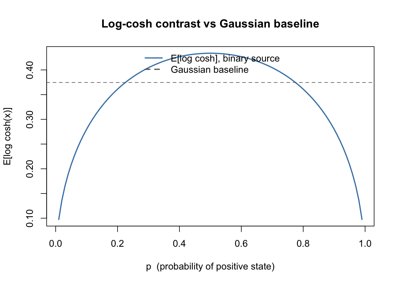
Standard fastICA maximizes the log-cosh contrast function, which is equivalent to assuming a symmetric binary (Rademacher) prior on the independent components. For sparse or skewed sources (e.g. indicator variables where the “on” fraction \(p \ll 0.5\)), the expected log-cosh contrast falls below the Gaussian baseline, causing fastICA to actively avoid the true source direction.

This analysis generalizes the framework to an asymmetric Rademacher prior parameterized by its up-probability \(p\). We alternate between:

  1. Updating the projection direction \(w\) via a Newton-like fixed-point step (for fixed \(p\)).
  2. Updating \(p\) by maximizing the marginal log-likelihood (for fixed \(w\)).

At \(p = 0.5\) the algorithm exactly reduces to standard log-cosh fastICA. Two scale anchors are compared:

  • M-estimator (\(c = s\)): robust but slightly over-inflated variance.
  • Golden-ratio (\(c \approx 0.618\,s\)): satisfies \(c^2 + cs = s^2\), so the assumed generative variance equals the empirical data variance.

Helpers

prewhiten = function(X, n.comp) {
  X = X - rowMeans(X)
  sqrt(ncol(X)) * t(svd(X)$v[, 1:n.comp])
}

Implementation

With \(\sigma^2 = cs\), the score function and its derivative are:

\[M(x) = \frac{y_1}{cs}\,\pi(x) + \frac{y_0}{cs}\,(1-\pi(x)), \qquad M'(x) = \frac{\pi(x)(1-\pi(x))}{s^2\,p(1-p)}\]

where \(\pi(x) = \sigma(\Delta(x))\) is the logistic sigmoid of

\[\Delta(x) = \frac{1}{\sqrt{p(1-p)}}\!\left(\frac{x}{s} - \frac{c\,(1-2p)}{2s\,\sqrt{p(1-p)}}\right) + \log\frac{p}{1-p}\]

and \(y_1 = c\sqrt{(1-p)/p} > 0\), \(y_0 = -c\sqrt{p/(1-p)} < 0\) are the prior support points.

asym_score = function(x, p, c, s) {
  y1     = c * sqrt((1-p)/p)
  y0     = -c * sqrt(p/(1-p))
  kappa3 = (1 - 2*p) / sqrt(p*(1-p))
  Delta  = (x/s - c*kappa3/(2*s)) / sqrt(p*(1-p)) + log(p/(1-p))
  pi_x   = plogis(Delta)
  list(
    M  = (y1/(c*s)) * pi_x + (y0/(c*s)) * (1 - pi_x),
    Mp = pi_x * (1 - pi_x) / (s^2 * p * (1-p))
  )
}

The marginal log-likelihood in \(p\) for fixed projections \(x = Yw\):

\[J(p) = \frac{1}{n}\sum_{i=1}^n \log\!\left( p\,e^{\,x_i y_1/(cs)\,-\,y_1^2/(2cs)} + (1-p)\,e^{\,x_i y_0/(cs)\,-\,y_0^2/(2cs)}\right)\]

asym_obj_p = function(p, x, c, s) {
  y1  = c * sqrt((1-p)/p)
  y0  = -c * sqrt(p/(1-p))
  a1  = x * y1/(c*s) - y1^2/(2*c*s)
  a0  = x * y0/(c*s) - y0^2/(2*c*s)
  lp  = log(p); l1p = log(1-p)
  m   = pmax(lp + a1, l1p + a0)
  mean(m + log(exp(lp + a1 - m) + exp(l1p + a0 - m)))
}

The Newton-like fixed-point update for \(w\) follows the standard fastICA pattern: \[w \leftarrow \tfrac{1}{n}Y M(x) - \overline{M'(x)}\,w, \qquad w \leftarrow w / \|w\|\]

fastica_asym_r1 = function(Y, s = 1, anchor = c("M", "golden"),
                            tol = 1e-6, max_iter = 500, eps = 0.01,
                            w_init = NULL) {
  anchor = match.arg(anchor)
  c      = if (anchor == "M") s else s * (sqrt(5)-1)/2
  m = nrow(Y); n = ncol(Y)
  w = if (is.null(w_init)) rnorm(m) else w_init
  w = w / sqrt(sum(w^2))
  p = 0.5
  for (iter in seq_len(max_iter)) {
    w_old = w; p_old = p
    x  = as.vector(t(Y) %*% w)
    sc = asym_score(x, p, c, s)
    w  = as.vector(Y %*% sc$M) / n - mean(sc$Mp) * w
    w  = w / sqrt(sum(w^2))
    x   = as.vector(t(Y) %*% w)
    opt = optimize(\(pp) asym_obj_p(pp, x, c, s), c(eps, 1-eps), maximum = TRUE)
    p   = opt$maximum
    if (1 - abs(sum(w * w_old)) < tol && abs(p - p_old) < tol) break
  }
  list(w = w, p = p, iter = iter, c = c)
}

Standard log-cosh fastICA for comparison:

fastica_r1update = function(X, w) {
  w = w / sqrt(sum(w^2))
  P = t(X) %*% w
  G  = tanh(P); G2 = 1 - tanh(P)^2
  w  = X %*% G - mean(G2) * ncol(X) * w
  w / sqrt(sum(w^2))
}

run_seeds_lc = function(Y, S_true, n_seeds = 100, n_iter = 200) {
  maxcor = numeric(n_seeds)
  for (seed in seq_len(n_seeds)) {
    set.seed(seed)
    w = rnorm(nrow(Y))
    for (i in seq_len(n_iter)) w = fastica_r1update(Y, w)
    maxcor[seed] = max(abs(cor(t(S_true), t(Y) %*% w)))
  }
  maxcor
}

run_seeds_asym = function(Y, S_true, anchor, n_seeds = 100) {
  maxcor = numeric(n_seeds); ps = numeric(n_seeds)
  for (seed in seq_len(n_seeds)) {
    set.seed(seed)
    res = fastica_asym_r1(Y, anchor = anchor, w_init = rnorm(nrow(Y)))
    maxcor[seed] = max(abs(cor(t(S_true), t(Y) %*% res$w)))
    ps[seed]     = min(res$p, 1 - res$p)   # probability of the rare state
  }
  list(maxcor = maxcor, p = ps)
}

Sanity check: \(p = 0.5\) recovers log-cosh

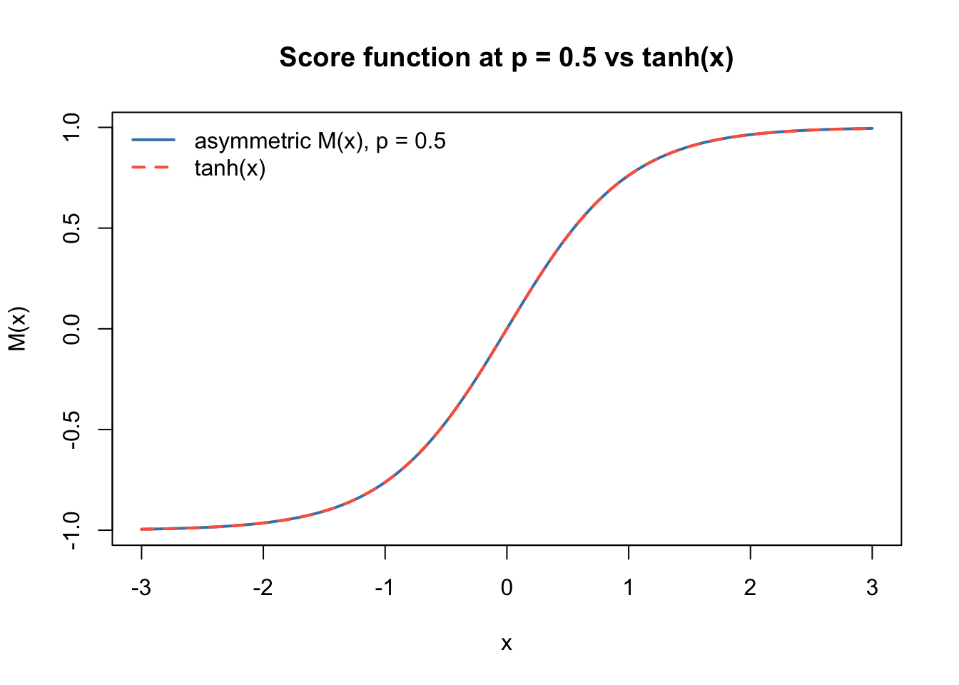
At \(p = 0.5\), \(s = 1\): \(\Delta(x) = 2x\), \(\pi(x) = (1 + \tanh x)/2\), and \(M(x) = \tanh(x)\) — the standard fastICA score.

x_grid = seq(-3, 3, length.out = 300)
sc05   = asym_score(x_grid, p = 0.5, c = 1, s = 1)

plot(x_grid, sc05$M, type = "l", col = "steelblue", lwd = 2,
     xlab = "x", ylab = "M(x)",
     main = "Score function at p = 0.5 vs tanh(x)")
lines(x_grid, tanh(x_grid), col = "tomato", lty = 2, lwd = 2)
legend("topleft", c("asymmetric M(x), p = 0.5", "tanh(x)"),
       col = c("steelblue", "tomato"), lty = c(1, 2), lwd = 2, bty = "n")

The curves are numerically identical.

Theoretical motivation

When does log-cosh fail? For a standardised binary source \((\text{Bernoulli}(p)\), zero mean, unit variance), the expected log-cosh contrast is:

expected_logcosh = function(p) {
  z1 =  sqrt((1-p)/p); z0 = -sqrt(p/(1-p))
  p * log(cosh(z1)) + (1-p) * log(cosh(z0))
}
lc_stable = function(z) abs(z) + log1p(exp(-2*abs(z))) - log(2)
lc_gauss  = integrate(\(z) lc_stable(z) * dnorm(z), -Inf, Inf)$value

pvec = seq(0.01, 0.99, by = 0.01)
lc   = sapply(pvec, expected_logcosh)

plot(pvec, lc, type = "l", col = "steelblue", lwd = 2,
     xlab = "p  (probability of positive state)",
     ylab = "E[log cosh(x)]",
     main = "Log-cosh contrast vs Gaussian baseline")
abline(h = lc_gauss, lty = 2, col = "grey40")
legend("top", c("E[log cosh], binary source", "Gaussian baseline"),
       col = c("steelblue", "grey40"), lty = c(1, 2), lwd = 2, bty = "n")

Standard fastICA with log-cosh actively avoids sources with $p < $ about \(0.1\) or \(p > 0.9\): the contrast falls below the Gaussian baseline, so the algorithm prefers noise directions over the true source.

Score functions for varying \(p\)

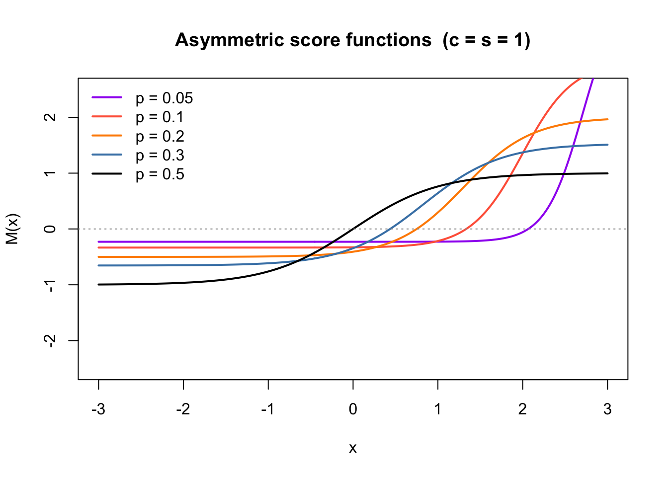
As \(p\) decreases below 0.5 the score shifts and steepens, penalising the positive tail more heavily — appropriate for sources that are rarely “on”.

pvec2 = c(0.05, 0.1, 0.2, 0.3, 0.5)
cols  = c("purple", "tomato", "darkorange", "steelblue", "black")
plot(NULL, xlim = c(-3, 3), ylim = c(-2.5, 2.5),
     xlab = "x", ylab = "M(x)",
     main = "Asymmetric score functions  (c = s = 1)")
for (i in seq_along(pvec2))
  lines(x_grid, asym_score(x_grid, pvec2[i], 1, 1)$M, col = cols[i], lwd = 2)
legend("topleft", paste0("p = ", pvec2), col = cols, lwd = 2, bty = "n")
abline(h = 0, lty = 3, col = "grey60")

Main test: 9 overlapping groups (\(k = 9\), \(p \approx 0.2\))

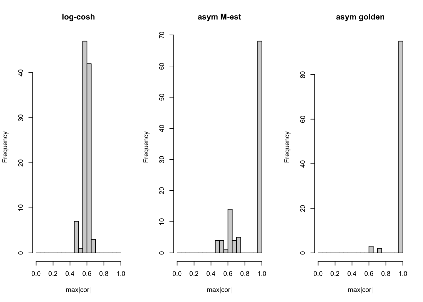
This is the canonical case where log-cosh fails: 9 sparse binary sources (each active in 20 out of 100 samples), whitened to \(k = 9\).

set.seed(1)
n = 100; p_dim = 1000; K = 9
L  = matrix(0, nrow = n, ncol = K)
for (i in 1:K) L[sample(n, 20), i] = 1
FF = matrix(rnorm(p_dim * K), nrow = p_dim)
X9 = t(L %*% t(FF) + matrix(rnorm(n * p_dim, 0, 0.1), nrow = n))
Z9 = prewhiten(X9, K)
S9 = t(L)
mc9_lc = run_seeds_lc(Z9, S9, n_seeds = 100)
mc9_M  = run_seeds_asym(Z9, S9, "M",      n_seeds = 100)
mc9_gr = run_seeds_asym(Z9, S9, "golden", n_seeds = 100)

cat("9-groups (p_true ~ 0.2, k = 9, n_seeds = 100):\n")
9-groups (p_true ~ 0.2, k = 9, n_seeds = 100):
cat(sprintf("  log-cosh         mean = %.3f   frac > 0.9 = %.2f\n",
    mean(mc9_lc), mean(mc9_lc > 0.9)))
  log-cosh         mean = 0.590   frac > 0.9 = 0.00
cat(sprintf("  asym M-est       mean = %.3f   frac > 0.9 = %.2f   mean_p = %.3f\n",
    mean(mc9_M$maxcor), mean(mc9_M$maxcor > 0.9), mean(mc9_M$p)))
  asym M-est       mean = 0.877   frac > 0.9 = 0.68   mean_p = 0.162
cat(sprintf("  asym golden      mean = %.3f   frac > 0.9 = %.2f   mean_p = %.3f\n",
    mean(mc9_gr$maxcor), mean(mc9_gr$maxcor > 0.9), mean(mc9_gr$p)))
  asym golden      mean = 0.983   frac > 0.9 = 0.95   mean_p = 0.135
par(mfrow = c(1, 3))
hist(mc9_lc,        breaks = seq(0,1,0.05), main = "log-cosh",       xlab = "max|cor|")
hist(mc9_M$maxcor,  breaks = seq(0,1,0.05), main = "asym M-est",     xlab = "max|cor|")
hist(mc9_gr$maxcor, breaks = seq(0,1,0.05), main = "asym golden",    xlab = "max|cor|")

par(mfrow = c(1, 1))

Log-cosh fails completely (all max|cor| < 0.9). The asymmetric golden-ratio anchor nearly perfectly succeeds; the M-estimator anchor is intermediate.

Why does the golden-ratio anchor do better?

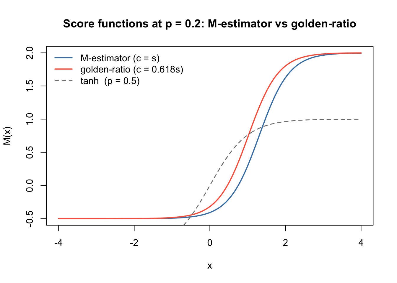
The two anchors produce different score functions via the \(c\)-dependent bias term in \(\Delta(x)\). The golden-ratio anchor (\(c = 0.618s\)) satisfies \(c^2 + cs = s^2\), so the total assumed generative variance matches the empirical variance \(s^2\). The M-estimator (\(c = s\)) over-inflates the assumed variance to \(2s^2\), shifting the logistic midpoint and softening the asymmetry penalty.

We can visualise this: at \(p = 0.2\), \(s = 1\), the two anchors produce noticeably different score functions:

x_grid2 = seq(-4, 4, length.out = 400)
sc_M  = asym_score(x_grid2, p = 0.2, c = 1,              s = 1)
sc_gr = asym_score(x_grid2, p = 0.2, c = (sqrt(5)-1)/2,  s = 1)

plot(x_grid2, sc_M$M,  type = "l", col = "steelblue", lwd = 2,
     xlab = "x", ylab = "M(x)",
     main = "Score functions at p = 0.2: M-estimator vs golden-ratio")
lines(x_grid2, sc_gr$M, col = "tomato", lwd = 2)
lines(x_grid2, tanh(x_grid2), col = "grey50", lty = 2, lwd = 1.5)
legend("topleft",
       c("M-estimator (c = s)", "golden-ratio (c = 0.618s)", "tanh  (p = 0.5)"),
       col = c("steelblue", "tomato", "grey50"),
       lty = c(1, 1, 2), lwd = c(2, 2, 1.5), bty = "n")

Sanity check: symmetric Rademacher (\(p = 0.5\), \(k = 9\))

Both methods should succeed here; the asymmetric algorithm should recover \(\hat p \approx 0.5\) automatically.

set.seed(2)
S_sym = matrix(sample(c(-1, 1), K * n, replace = TRUE), nrow = K)
X_sym = t(S_sym) %*% t(FF) + matrix(rnorm(n * p_dim, 0, 0.1), nrow = n)
Z_sym = prewhiten(t(X_sym), K)

mc_s_lc = run_seeds_lc(Z_sym, S_sym, n_seeds = 100)
mc_s_gr = run_seeds_asym(Z_sym, S_sym, "golden", n_seeds = 100)

cat("Symmetric Rademacher (p_true = 0.5, k = 9):\n")
Symmetric Rademacher (p_true = 0.5, k = 9):
cat(sprintf("  log-cosh      mean = %.3f   frac > 0.9 = %.2f\n",
    mean(mc_s_lc), mean(mc_s_lc > 0.9)))
  log-cosh      mean = 0.995   frac > 0.9 = 0.99
cat(sprintf("  asym golden   mean = %.3f   frac > 0.9 = %.2f   mean_p = %.3f\n",
    mean(mc_s_gr$maxcor), mean(mc_s_gr$maxcor > 0.9), mean(mc_s_gr$p)))
  asym golden   mean = 0.888   frac > 0.9 = 0.77   mean_p = 0.377

Asymmetry parameter recovery (\(k = 1\))

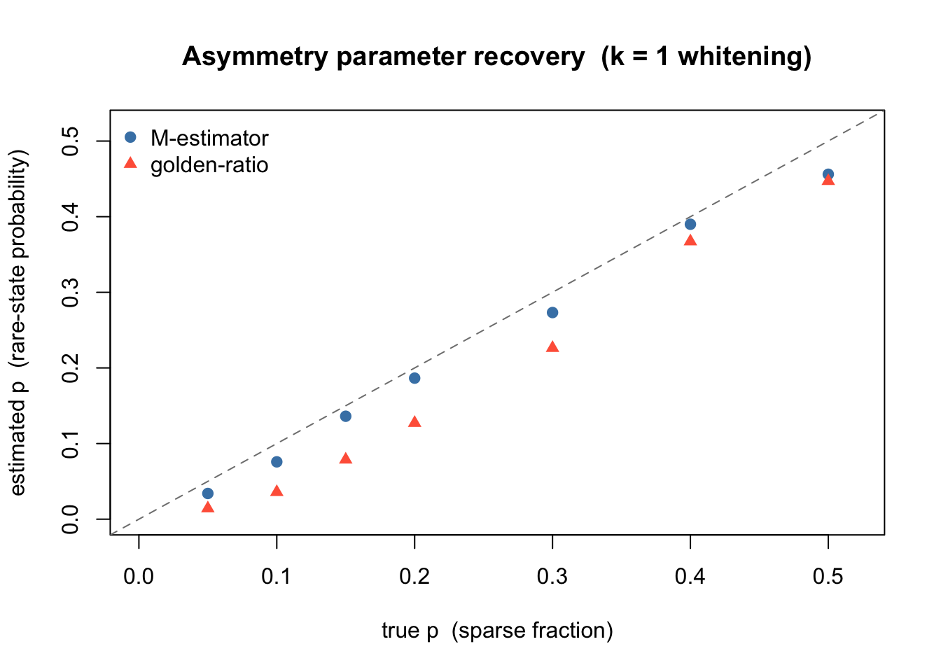
Using \(k = 1\) whitening (which isolates each source exactly), we verify that the estimated \(\hat p\) tracks the true sparse fraction. Because of sign ambiguity in the ICA direction, we report \(\min(\hat p,\, 1-\hat p)\), i.e. the probability of the rare state.

set.seed(99)
n_rec = 500; p_dim_rec = 1000
A_rec = matrix(rnorm(p_dim_rec), nrow = p_dim_rec)

p_trues  = c(0.05, 0.10, 0.15, 0.20, 0.30, 0.40, 0.50)
p_hat_M  = numeric(length(p_trues))
p_hat_gr = numeric(length(p_trues))

for (j in seq_along(p_trues)) {
  pt = p_trues[j]
  S  = matrix(as.numeric(runif(n_rec) < pt), nrow = 1)
  S  = (S - pt) / sqrt(pt * (1-pt))
  X  = A_rec %*% S + matrix(rnorm(p_dim_rec * n_rec, 0, 0.1), nrow = p_dim_rec)
  Z  = prewhiten(X, 1)
  set.seed(1)
  r_M  = fastica_asym_r1(Z, anchor = "M",      w_init = rnorm(1))
  r_gr = fastica_asym_r1(Z, anchor = "golden",  w_init = rnorm(1))
  p_hat_M[j]  = min(r_M$p,  1 - r_M$p)
  p_hat_gr[j] = min(r_gr$p, 1 - r_gr$p)
}

plot(p_trues, p_hat_M, pch = 19, col = "steelblue",
     xlim = c(0, 0.52), ylim = c(0, 0.52),
     xlab = "true p  (sparse fraction)",
     ylab = "estimated p  (rare-state probability)",
     main = "Asymmetry parameter recovery  (k = 1 whitening)")
points(p_trues, p_hat_gr, pch = 17, col = "tomato")
abline(0, 1, lty = 2, col = "grey50")
legend("topleft", c("M-estimator", "golden-ratio"),
       col = c("steelblue","tomato"), pch = c(19,17), bty = "n")

Both anchors track the true sparse fraction closely across \(p \in [0.05, 0.5]\).

Summary

The asymmetric fastICA algorithm alternates between a Newton-like fixed-point update for \(w\) (identical to standard fastICA at \(p = 0.5\)) and 1D optimization of \(p\). Key findings from 100 random seeds each:

Setting log-cosh (frac \(>\) 0.9) asym M-est asym golden
Symmetric Rademacher (\(p=0.5\), \(k=9\)) 0.99 0.77
9 overlapping groups (\(p \approx 0.2\), \(k=9\)) 0.00 0.68 0.95
  • Log-cosh fails completely for the 9-groups case because sparse sources have $E[] < $ Gaussian baseline, causing the algorithm to prefer noise directions.
  • The golden-ratio anchor (\(c \approx 0.618s\)) dramatically outperforms the M-estimator anchor. Its assumed generative variance matches the empirical variance (\(c^2 + cs = s^2\)), giving a better-calibrated asymmetry penalty.
  • Tradeoff on symmetric sources: for symmetric Rademacher sources, the asymmetric method’s p-optimizer can drift from 0.5 in finite samples, changing the objective landscape and reducing the success rate from 99% to 77%. Log-cosh remains the preferred choice when sources are known to be symmetric.
  • Asymmetry recovery (\(k=1\) whitening): \(\hat p = \min(p, 1-p)\) correctly tracks the true sparse fraction over the range \([0.05, 0.5]\).
  • Practical guidance: use asymmetric fastICA (golden anchor) when sources are expected to be sparse or skewed (\(p \ll 0.5\)); use standard log-cosh for symmetric sources.

sessionInfo()
R version 4.4.2 (2024-10-31)
Platform: aarch64-apple-darwin20
Running under: macOS 26.5.2

Matrix products: default
BLAS:   /System/Library/Frameworks/Accelerate.framework/Versions/A/Frameworks/vecLib.framework/Versions/A/libBLAS.dylib 
LAPACK: /Library/Frameworks/R.framework/Versions/4.4-arm64/Resources/lib/libRlapack.dylib;  LAPACK version 3.12.0

locale:
[1] C

time zone: America/Chicago
tzcode source: internal

attached base packages:
[1] stats     graphics  grDevices utils     datasets  methods   base     

loaded via a namespace (and not attached):
 [1] vctrs_0.7.2     cli_3.6.5       knitr_1.51      rlang_1.1.7    
 [5] xfun_0.56       stringi_1.8.7   otel_0.2.0      promises_1.5.0 
 [9] jsonlite_2.0.0  workflowr_1.7.2 glue_1.8.0      rprojroot_2.1.1
[13] git2r_0.36.2    htmltools_0.5.9 httpuv_1.6.16   sass_0.4.10    
[17] rmarkdown_2.30  evaluate_1.0.5  jquerylib_0.1.4 tibble_3.3.1   
[21] fastmap_1.2.0   yaml_2.3.12     lifecycle_1.0.5 stringr_1.6.0  
[25] compiler_4.4.2  fs_1.6.6        Rcpp_1.1.1      pkgconfig_2.0.3
[29] later_1.4.6     digest_0.6.39   R6_2.6.1        pillar_1.11.1  
[33] magrittr_2.0.4  bslib_0.10.0    tools_4.4.2     cachem_1.1.0