fastica_centered_02
Matthew Stephens
2025-11-18
Last updated: 2025-11-20
Checks: 7 0
Knit directory: misc/analysis/
This reproducible R Markdown analysis was created with workflowr (version 1.7.1). The Checks tab describes the reproducibility checks that were applied when the results were created. The Past versions tab lists the development history.
Great! Since the R Markdown file has been committed to the Git repository, you know the exact version of the code that produced these results.
Great job! The global environment was empty. Objects defined in the global environment can affect the analysis in your R Markdown file in unknown ways. For reproduciblity it’s best to always run the code in an empty environment.
The command set.seed(1) was run prior to running the
code in the R Markdown file. Setting a seed ensures that any results
that rely on randomness, e.g. subsampling or permutations, are
reproducible.
Great job! Recording the operating system, R version, and package versions is critical for reproducibility.
Nice! There were no cached chunks for this analysis, so you can be confident that you successfully produced the results during this run.
Great job! Using relative paths to the files within your workflowr project makes it easier to run your code on other machines.
Great! You are using Git for version control. Tracking code development and connecting the code version to the results is critical for reproducibility.
The results in this page were generated with repository version 17f6fd7. See the Past versions tab to see a history of the changes made to the R Markdown and HTML files.
Note that you need to be careful to ensure that all relevant files for
the analysis have been committed to Git prior to generating the results
(you can use wflow_publish or
wflow_git_commit). workflowr only checks the R Markdown
file, but you know if there are other scripts or data files that it
depends on. Below is the status of the Git repository when the results
were generated:
Ignored files:
    Ignored:    .DS_Store
    Ignored:    .Rhistory
    Ignored:    .Rproj.user/
    Ignored:    analysis/.RData
    Ignored:    analysis/.Rhistory
    Ignored:    analysis/ALStruct_cache/
    Ignored:    data/.Rhistory
    Ignored:    data/methylation-data-for-matthew.rds
    Ignored:    data/pbmc/
    Ignored:    data/pbmc_purified.RData

Untracked files:
    Untracked:  .dropbox
    Untracked:  Icon
    Untracked:  analysis/GHstan.Rmd
    Untracked:  analysis/GTEX-cogaps.Rmd
    Untracked:  analysis/PACS.Rmd
    Untracked:  analysis/Rplot.png
    Untracked:  analysis/SPCAvRP.rmd
    Untracked:  analysis/abf_comparisons.Rmd
    Untracked:  analysis/admm_02.Rmd
    Untracked:  analysis/admm_03.Rmd
    Untracked:  analysis/bispca.Rmd
    Untracked:  analysis/cache/
    Untracked:  analysis/cholesky.Rmd
    Untracked:  analysis/compare-transformed-models.Rmd
    Untracked:  analysis/cormotif.Rmd
    Untracked:  analysis/cp_ash.Rmd
    Untracked:  analysis/eQTL.perm.rand.pdf
    Untracked:  analysis/eb_power2.Rmd
    Untracked:  analysis/eb_prepilot.Rmd
    Untracked:  analysis/eb_var.Rmd
    Untracked:  analysis/ebpmf1.Rmd
    Untracked:  analysis/ebpmf_sla_text.Rmd
    Untracked:  analysis/ebspca_sims.Rmd
    Untracked:  analysis/explore_psvd.Rmd
    Untracked:  analysis/fa_check_identify.Rmd
    Untracked:  analysis/fa_iterative.Rmd
    Untracked:  analysis/fastica_centered_03.Rmd
    Untracked:  analysis/fastica_heated.Rmd
    Untracked:  analysis/flash_cov_overlapping_groups_init.Rmd
    Untracked:  analysis/flash_test_tree.Rmd
    Untracked:  analysis/flashier_newgroups.Rmd
    Untracked:  analysis/flashier_nmf_triples.Rmd
    Untracked:  analysis/flashier_pbmc.Rmd
    Untracked:  analysis/flashier_snn_shifted_prior.Rmd
    Untracked:  analysis/greedy_ebpmf_exploration_00.Rmd
    Untracked:  analysis/ieQTL.perm.rand.pdf
    Untracked:  analysis/lasso_em_03.Rmd
    Untracked:  analysis/m6amash.Rmd
    Untracked:  analysis/mash_bhat_z.Rmd
    Untracked:  analysis/mash_ieqtl_permutations.Rmd
    Untracked:  analysis/methylation_example.Rmd
    Untracked:  analysis/mixsqp.Rmd
    Untracked:  analysis/mr.ash_lasso_init.Rmd
    Untracked:  analysis/mr.mash.test.Rmd
    Untracked:  analysis/mr_ash_modular.Rmd
    Untracked:  analysis/mr_ash_parameterization.Rmd
    Untracked:  analysis/mr_ash_ridge.Rmd
    Untracked:  analysis/mv_gaussian_message_passing.Rmd
    Untracked:  analysis/nejm.Rmd
    Untracked:  analysis/nmf_bg.Rmd
    Untracked:  analysis/nonneg_underapprox.Rmd
    Untracked:  analysis/normal_conditional_on_r2.Rmd
    Untracked:  analysis/normalize.Rmd
    Untracked:  analysis/pbmc.Rmd
    Untracked:  analysis/pca_binary_weighted.Rmd
    Untracked:  analysis/pca_l1.Rmd
    Untracked:  analysis/poisson_nmf_approx.Rmd
    Untracked:  analysis/poisson_shrink.Rmd
    Untracked:  analysis/poisson_transform.Rmd
    Untracked:  analysis/qrnotes.txt
    Untracked:  analysis/ridge_iterative_02.Rmd
    Untracked:  analysis/ridge_iterative_splitting.Rmd
    Untracked:  analysis/samps/
    Untracked:  analysis/sc_bimodal.Rmd
    Untracked:  analysis/shrinkage_comparisons_changepoints.Rmd
    Untracked:  analysis/susie_cov.Rmd
    Untracked:  analysis/susie_en.Rmd
    Untracked:  analysis/susie_z_investigate.Rmd
    Untracked:  analysis/svd-timing.Rmd
    Untracked:  analysis/temp.RDS
    Untracked:  analysis/temp.Rmd
    Untracked:  analysis/test-figure/
    Untracked:  analysis/test.Rmd
    Untracked:  analysis/test.Rpres
    Untracked:  analysis/test.md
    Untracked:  analysis/test_qr.R
    Untracked:  analysis/test_sparse.Rmd
    Untracked:  analysis/tree_dist_top_eigenvector.Rmd
    Untracked:  analysis/z.txt
    Untracked:  code/coordinate_descent_symNMF.R
    Untracked:  code/multivariate_testfuncs.R
    Untracked:  code/rqb.hacked.R
    Untracked:  data/4matthew/
    Untracked:  data/4matthew2/
    Untracked:  data/E-MTAB-2805.processed.1/
    Untracked:  data/ENSG00000156738.Sim_Y2.RDS
    Untracked:  data/GDS5363_full.soft.gz
    Untracked:  data/GSE41265_allGenesTPM.txt
    Untracked:  data/Muscle_Skeletal.ACTN3.pm1Mb.RDS
    Untracked:  data/P.rds
    Untracked:  data/Thyroid.FMO2.pm1Mb.RDS
    Untracked:  data/bmass.HaemgenRBC2016.MAF01.Vs2.MergedDataSources.200kRanSubset.ChrBPMAFMarkerZScores.vs1.txt.gz
    Untracked:  data/bmass.HaemgenRBC2016.Vs2.NewSNPs.ZScores.hclust.vs1.txt
    Untracked:  data/bmass.HaemgenRBC2016.Vs2.PreviousSNPs.ZScores.hclust.vs1.txt
    Untracked:  data/eb_prepilot/
    Untracked:  data/finemap_data/fmo2.sim/b.txt
    Untracked:  data/finemap_data/fmo2.sim/dap_out.txt
    Untracked:  data/finemap_data/fmo2.sim/dap_out2.txt
    Untracked:  data/finemap_data/fmo2.sim/dap_out2_snp.txt
    Untracked:  data/finemap_data/fmo2.sim/dap_out_snp.txt
    Untracked:  data/finemap_data/fmo2.sim/data
    Untracked:  data/finemap_data/fmo2.sim/fmo2.sim.config
    Untracked:  data/finemap_data/fmo2.sim/fmo2.sim.k
    Untracked:  data/finemap_data/fmo2.sim/fmo2.sim.k4.config
    Untracked:  data/finemap_data/fmo2.sim/fmo2.sim.k4.snp
    Untracked:  data/finemap_data/fmo2.sim/fmo2.sim.ld
    Untracked:  data/finemap_data/fmo2.sim/fmo2.sim.snp
    Untracked:  data/finemap_data/fmo2.sim/fmo2.sim.z
    Untracked:  data/finemap_data/fmo2.sim/pos.txt
    Untracked:  data/logm.csv
    Untracked:  data/m.cd.RDS
    Untracked:  data/m.cdu.old.RDS
    Untracked:  data/m.new.cd.RDS
    Untracked:  data/m.old.cd.RDS
    Untracked:  data/mainbib.bib.old
    Untracked:  data/mat.csv
    Untracked:  data/mat.txt
    Untracked:  data/mat_new.csv
    Untracked:  data/matrix_lik.rds
    Untracked:  data/paintor_data/
    Untracked:  data/running_data_chris.csv
    Untracked:  data/running_data_matthew.csv
    Untracked:  data/temp.txt
    Untracked:  data/y.txt
    Untracked:  data/y_f.txt
    Untracked:  data/zscore_jointLCLs_m6AQTLs_susie_eQTLpruned.rds
    Untracked:  data/zscore_jointLCLs_random.rds
    Untracked:  explore_udi.R
    Untracked:  output/fit.k10.rds
    Untracked:  output/fit.nn.pbmc.purified.rds
    Untracked:  output/fit.nn.rds
    Untracked:  output/fit.nn.s.001.rds
    Untracked:  output/fit.nn.s.01.rds
    Untracked:  output/fit.nn.s.1.rds
    Untracked:  output/fit.nn.s.10.rds
    Untracked:  output/fit.snn.s.001.rds
    Untracked:  output/fit.snn.s.01.nninit.rds
    Untracked:  output/fit.snn.s.01.rds
    Untracked:  output/fit.varbvs.RDS
    Untracked:  output/fit2.nn.pbmc.purified.rds
    Untracked:  output/glmnet.fit.RDS
    Untracked:  output/snn07.txt
    Untracked:  output/snn34.txt
    Untracked:  output/test.bv.txt
    Untracked:  output/test.gamma.txt
    Untracked:  output/test.hyp.txt
    Untracked:  output/test.log.txt
    Untracked:  output/test.param.txt
    Untracked:  output/test2.bv.txt
    Untracked:  output/test2.gamma.txt
    Untracked:  output/test2.hyp.txt
    Untracked:  output/test2.log.txt
    Untracked:  output/test2.param.txt
    Untracked:  output/test3.bv.txt
    Untracked:  output/test3.gamma.txt
    Untracked:  output/test3.hyp.txt
    Untracked:  output/test3.log.txt
    Untracked:  output/test3.param.txt
    Untracked:  output/test4.bv.txt
    Untracked:  output/test4.gamma.txt
    Untracked:  output/test4.hyp.txt
    Untracked:  output/test4.log.txt
    Untracked:  output/test4.param.txt
    Untracked:  output/test5.bv.txt
    Untracked:  output/test5.gamma.txt
    Untracked:  output/test5.hyp.txt
    Untracked:  output/test5.log.txt
    Untracked:  output/test5.param.txt

Unstaged changes:
    Modified:   .gitignore
    Modified:   analysis/eb_snmu.Rmd
    Modified:   analysis/ebnm_binormal.Rmd
    Modified:   analysis/ebpower.Rmd
    Modified:   analysis/fastica_centered.Rmd
    Modified:   analysis/flashier_log1p.Rmd
    Modified:   analysis/flashier_sla_text.Rmd
    Modified:   analysis/logistic_z_scores.Rmd
    Modified:   analysis/mr_ash_pen.Rmd
    Modified:   analysis/nmu_em.Rmd
    Modified:   analysis/susie_flash.Rmd
    Modified:   analysis/tap_free_energy.Rmd
    Modified:   misc.Rproj
Note that any generated files, e.g. HTML, png, CSS, etc., are not included in this status report because it is ok for generated content to have uncommitted changes.
These are the previous versions of the repository in which changes were
made to the R Markdown (analysis/fastica_centered_02.Rmd)
and HTML (docs/fastica_centered_02.html) files. If you’ve
configured a remote Git repository (see ?wflow_git_remote),
click on the hyperlinks in the table below to view the files as they
were in that past version.
| File | Version | Author | Date | Message |
|---|---|---|---|---|
| Rmd | 17f6fd7 | Matthew Stephens | 2025-11-20 | workflowr::wflow_publish("fastica_centered_02.Rmd") |
| html | cbf04fa | Matthew Stephens | 2025-11-18 | Build site. |
| Rmd | 882882a | Matthew Stephens | 2025-11-18 | workflowr::wflow_publish("fastica_centered_02.Rmd") |
Introduction
I found previously that the original fastICA algorithm seems to have trouble finding groups that are unbalanced. I believe that this is because the log-cosh objective function favours symmetry. ie maximizing or minimizing \(\log \cosh (X'w)\) (subject to \(w'w=1\), which implies ||X’w||= 1 if \(XX'=I\)) tends to find symmetric \(X'w\). I want to try to fix this using an intercept. That is, maximize \(\log \cosh (X'w + c)\) over both \(w\) and \(c\). I made an initial attempt but I now believe that was flawed. The issue is that simply adding in a c makes the objective unbounded, and I actually ended up minimising over c while maximising over w, which is a mess. Here I’m going to try a different approach, which simply constriains ||X’w + c||=1, which is equivalent to adding a row of 1s to the whitened matrix X.
Illustrating the problem
Before trying to fix the problem, let’s illustrate it again. First here is a simple single-unit ICA function and preprocessing (for centering and whitening).
fastica_r1update = function(X,w, includeG2=TRUE){
  w= w/sqrt(sum(w^2)) # redundant, but just to be safe
  P = t(X) %*% w
  G = tanh(P)
  G2 = 0
  if(includeG2) # Note: if you don't include G2, this is like the EBCD updates rather than ICA and I believe it will always try to maximize logcosh
    G2 = 1-tanh(P)^2

  w = X %*% G - sum(G2) * w
  w = w/sqrt(sum(w^2)) # to ensure the returned value satisfies constraints
  return(w)
}


preprocess = function(X, n.comp=10){
  n <- nrow(X)
  p <- ncol(X)
  X <- scale(X, scale = FALSE)
  X <- t(X)

  ## This appears to be equivalant to X1 = t(svd(X)$v[,1:n.comp])
  V <- X %*% t(X)/n
  s <- La.svd(V)
  D <- diag(c(1/sqrt(s$d)))
  K <- D %*% t(s$u)
  K <- matrix(K[1:n.comp, ], n.comp, p)
  X1 <- K %*% X
  return(X1)
}

compute_objective = function(X,w){
  P = t(X) %*% w
  return(mean(log(cosh(P))))
}
Three group simulation
Here I simulate 3 groups, with only 20 members each.
K=3
p = 1000
n = 100
set.seed(1)
L = matrix(-1,nrow=n,ncol=K)
for(i in 1:K){L[sample(1:n,20),i]=1}
FF = matrix(rnorm(p*K), nrow = p, ncol=K)

X = L %*% t(FF) + rnorm(n*p,0,0.01)
plot(X %*% FF[,1])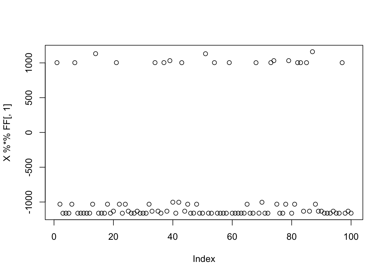
| Version | Author | Date |
|---|---|---|
| cbf04fa | Matthew Stephens | 2025-11-18 |
X1 = preprocess(X)fastICA
Running single unit fastICA on these data does not pick out a single source:
w = rnorm(nrow(X1))
for(i in 1:100)
  w = fastica_r1update(X1,w)
cor(L,t(X1) %*% w)
[,1]
[1,] -0.09720849
[2,] 0.39491239
[3,] 0.06322010plot(t(X1) %*% w)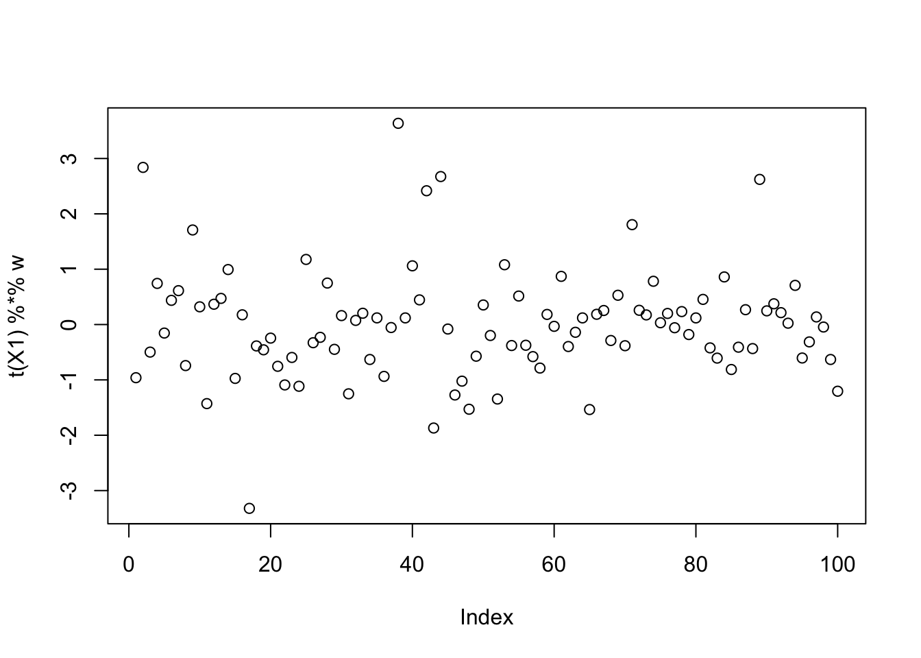
| Version | Author | Date |
|---|---|---|
| cbf04fa | Matthew Stephens | 2025-11-18 |
compute_objective(X1,w)[1] 0.3320872Try initializing near a true source. Note that the initialization, because everything is centered, is mean 0, but because it is so skew it is not “centered” on 0. Furthermore, its expected log(cosh) value is close to a Gaussian even though this source is very non-gaussian!
init_w = X1 %*% L[,1]
init_w = init_w/sqrt(sum(init_w^2))
plot(t(X1) %*% init_w,main="initial value of source estimate")
abline(h=0)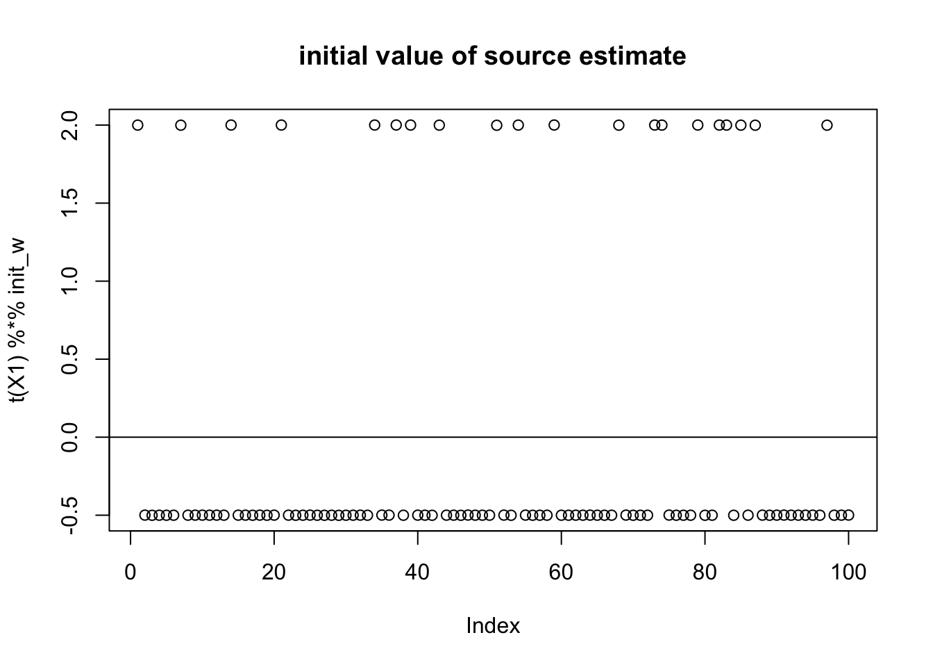
| Version | Author | Date |
|---|---|---|
| cbf04fa | Matthew Stephens | 2025-11-18 |
compute_objective(X1,init_w)[1] 0.3610922mean(log(cosh(rnorm(10000)))) # expected logcosh for normal[1] 0.3682596Running fastICA from this initialization finds something with a larger objective, but actually more “gaussian”. This indicates that the objective function is not doing what we want.
w = init_w
for(i in 1:100)
  w = fastica_r1update(X1,w)
cor(L,t(X1) %*% w)
[,1]
[1,] -0.189724426
[2,] 0.087759754
[3,] 0.008005984plot(t(X1) %*% w)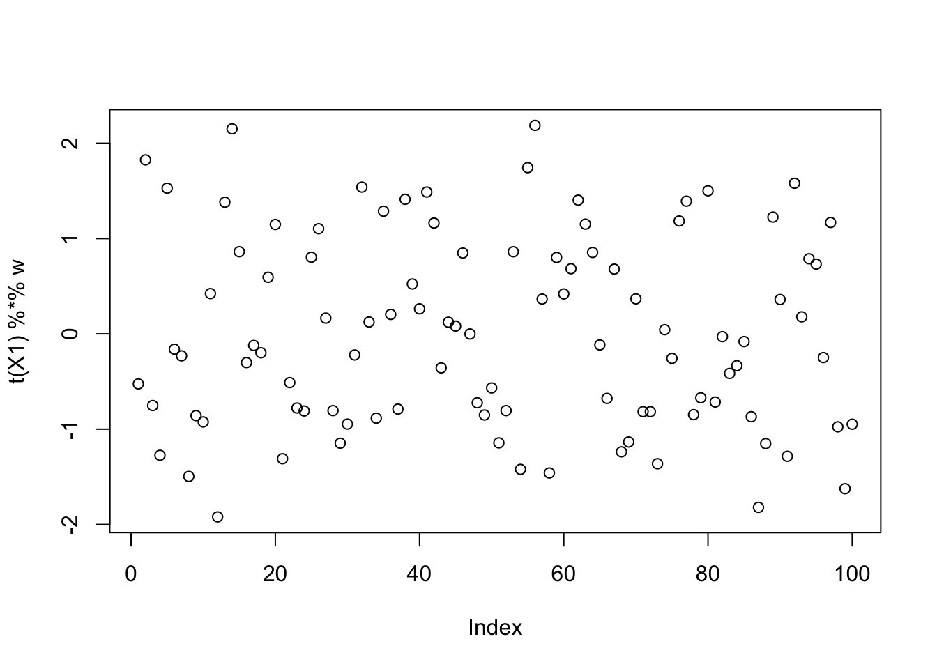
| Version | Author | Date |
|---|---|---|
| cbf04fa | Matthew Stephens | 2025-11-18 |
compute_objective(X1,w)[1] 0.3958629Attempt to fix the problem: noncentered fastICA
Here I attempt to fix the problem by adding an intercept to create a “noncentered” version of fastICA. We do this simply by adding a row of 1s to X1. Note that the resulting augmented X1 is still whitened (X1 X1’ is nI).
X1 = rbind(X1, rep(1,ncol(X1)))
image(X1 %*% t(X1))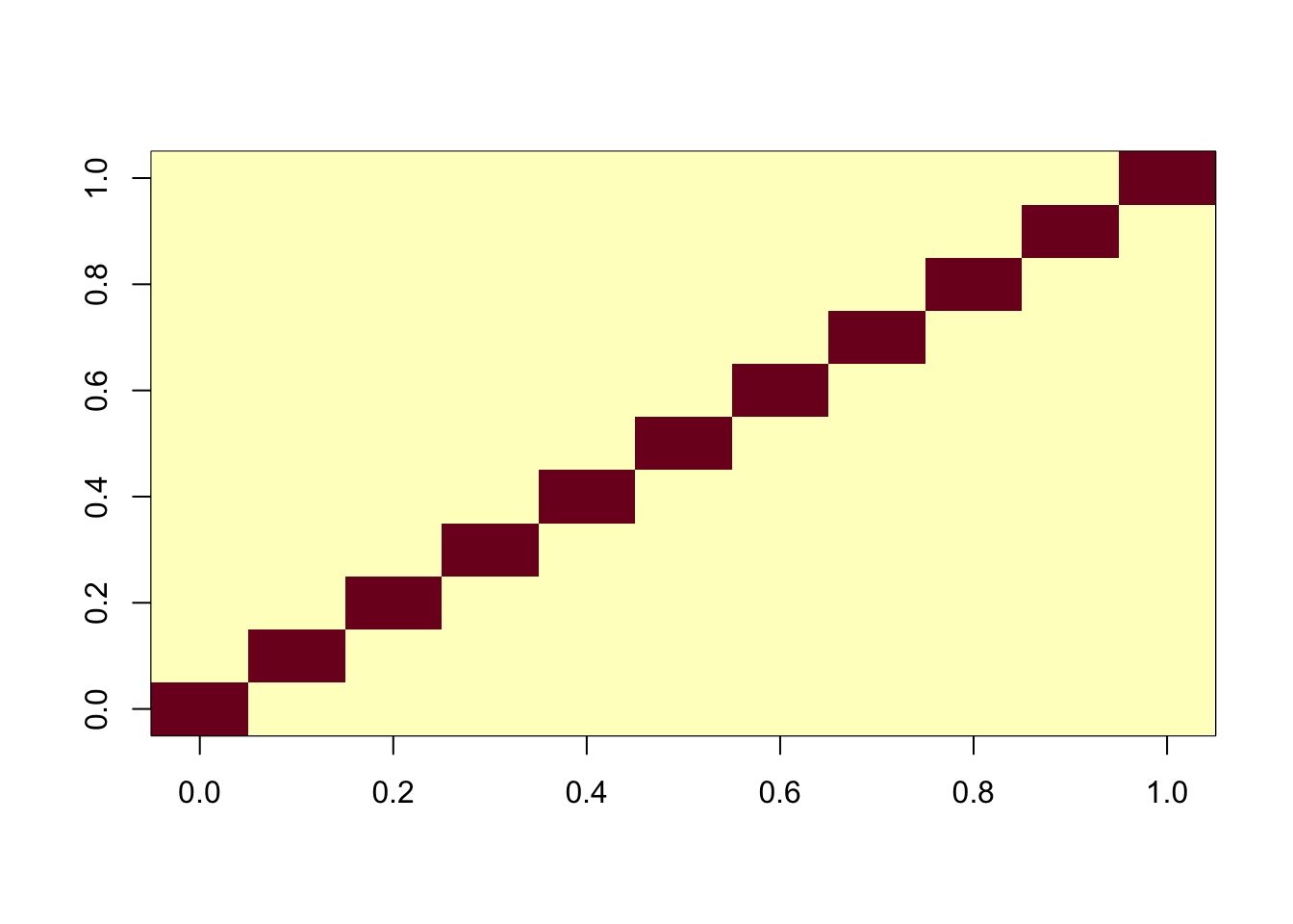
| Version | Author | Date |
|---|---|---|
| cbf04fa | Matthew Stephens | 2025-11-18 |
Initialize again near the true source: note that now the initial source is “centered” at 0 (but it is not mean 0). It is very close to a binary distribution on -1,1 which maximizes expected log(cosh) subject to the second moment constraint.
init_w = X1 %*% L[,1]
init_w = init_w/sqrt(sum(init_w^2))
plot(t(X1) %*% init_w,main="initial value of source estimate")
abline(h=0)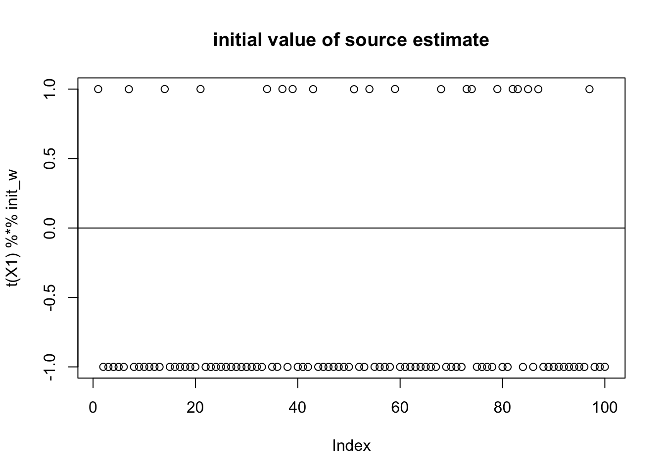
| Version | Author | Date |
|---|---|---|
| cbf04fa | Matthew Stephens | 2025-11-18 |
compute_objective(X1,init_w)[1] 0.4337808Running fastICA from this initialization now finds the correct source!
w = init_w
for(i in 1:100)
  w = fastica_r1update(X1,w)
cor(L,t(X1) %*% w)
[,1]
[1,] 9.999999e-01
[2,] 1.770293e-08
[3,] -6.250002e-02plot(t(X1) %*% w)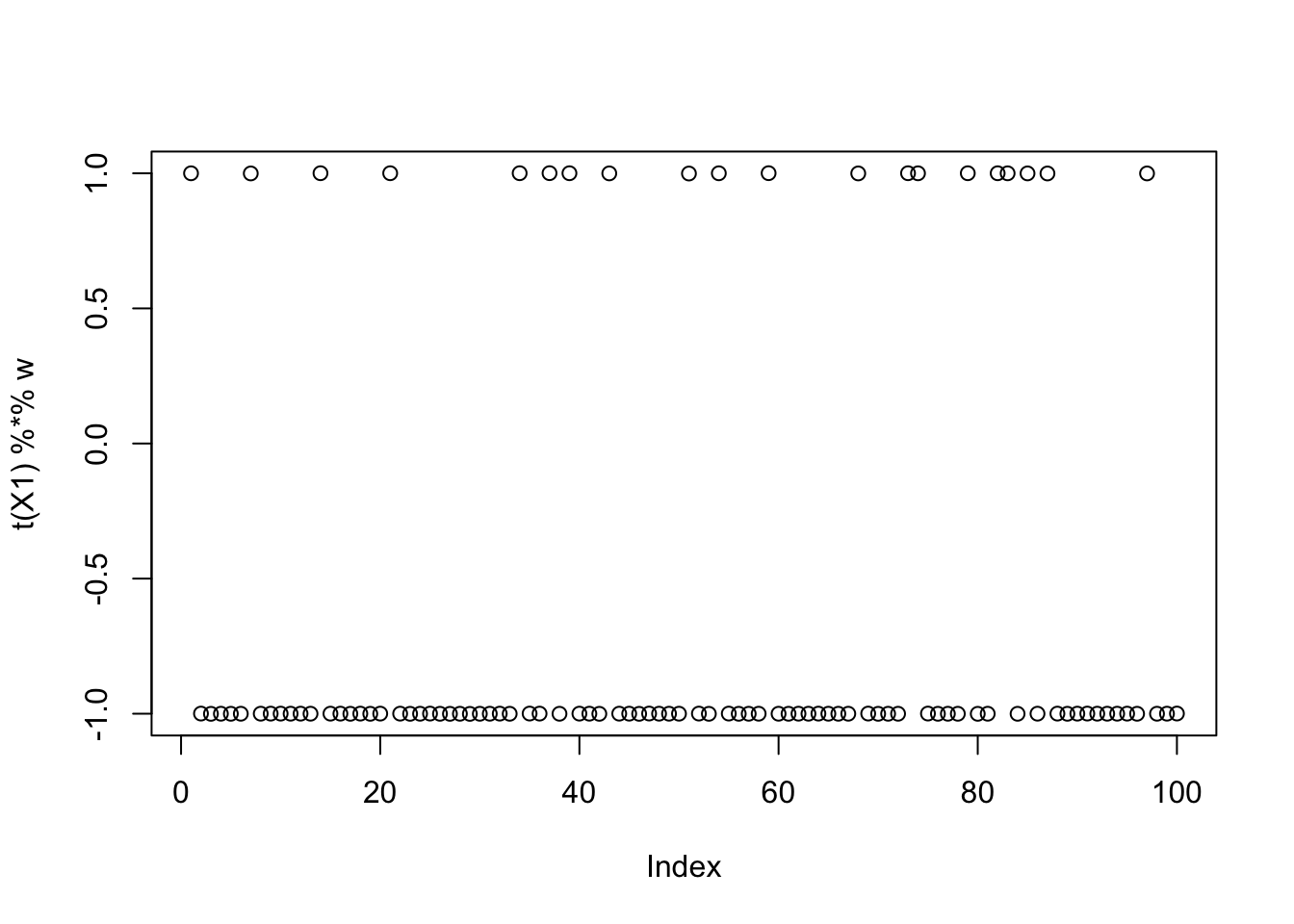
| Version | Author | Date |
|---|---|---|
| cbf04fa | Matthew Stephens | 2025-11-18 |
compute_objective(X1,w)[1] 0.4337808Running fastICA from a random initialization also finds a binary source:
w = rnorm(nrow(X1))
for(i in 1:100)
  w = fastica_r1update(X1,w)
cor(L,t(X1) %*% w)
[,1]
[1,] 1.041264e-08
[2,] 9.999999e-01
[3,] 5.026142e-09plot(t(X1) %*% w)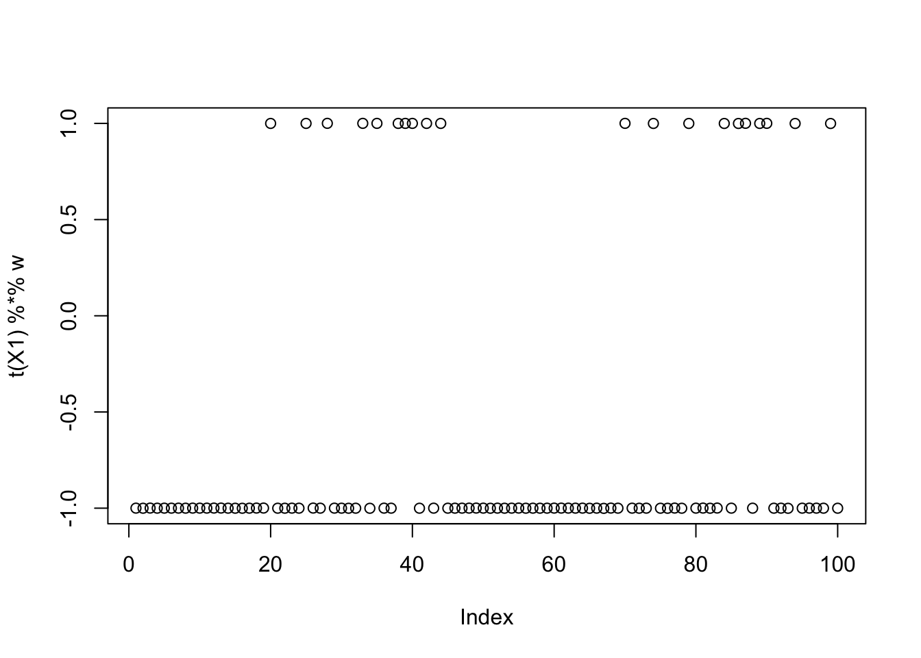
| Version | Author | Date |
|---|---|---|
| cbf04fa | Matthew Stephens | 2025-11-18 |
compute_objective(X1,w)[1] 0.4337808Here I run from 100 different random seeds. Most runs appear to find a binary source with objective around 0.44. But a good fraction find ones with small objective around 0.3, presumably corresponding to a minima (or local minima) of the objective.
obj = rep(0,100)
for(seed in 1:100){
  set.seed(seed)
  w = rnorm(nrow(X1))
  for(i in 1:100)
    w = fastica_r1update(X1,w)
  obj[seed] = compute_objective(X1,w)
}
plot(obj)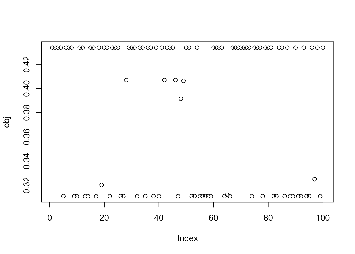
| Version | Author | Date |
|---|---|---|
| cbf04fa | Matthew Stephens | 2025-11-18 |
Interestingly the small values are also binary sources. Here is the seed with the smallest objective:
seed = which.min(obj)
set.seed(seed)
w = rnorm(nrow(X1))
for(i in 1:100)
  w = fastica_r1update(X1,w)
plot(t(X1) %*% w)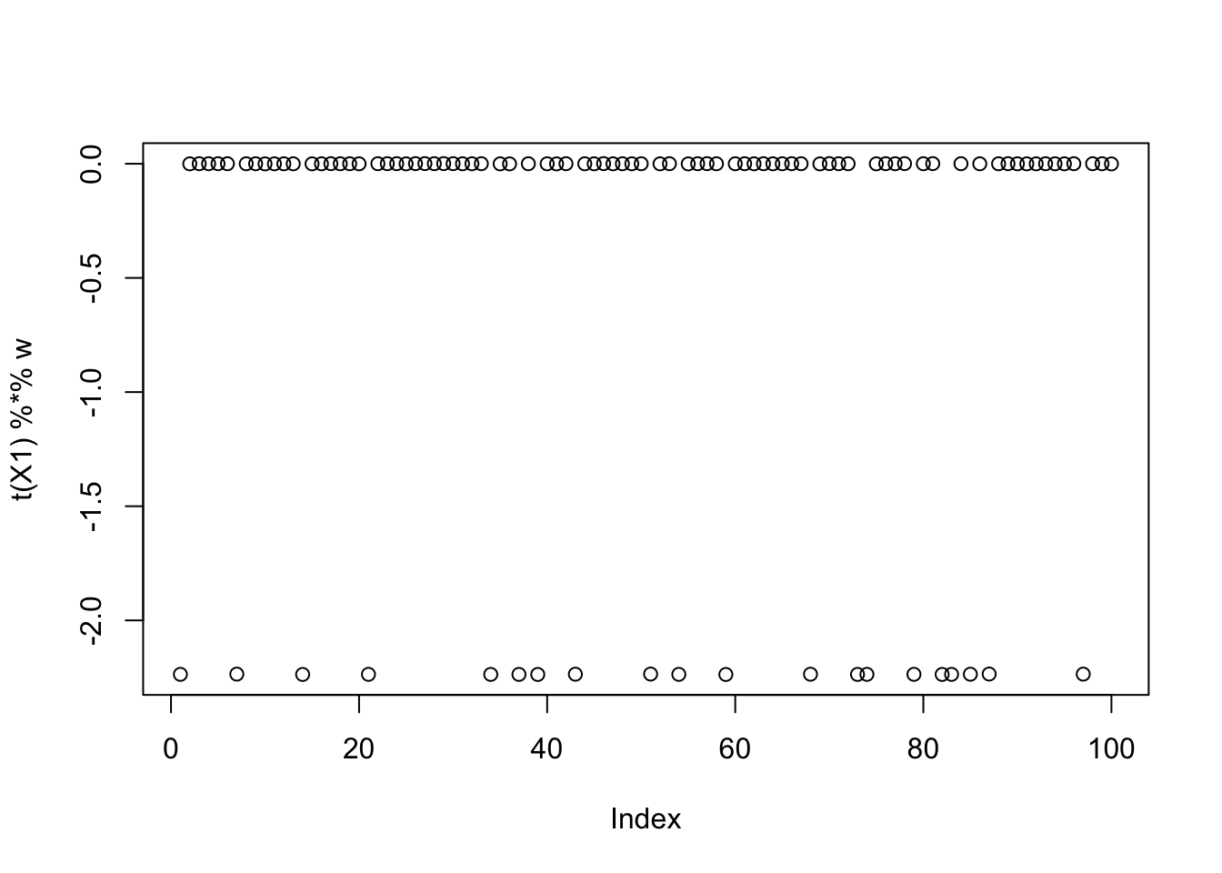
| Version | Author | Date |
|---|---|---|
| cbf04fa | Matthew Stephens | 2025-11-18 |
cor(L, t(X1) %*% w) [,1]
[1,] -9.999999e-01
[2,] 1.128688e-05
[3,] 6.257773e-02So: what is going on here is that there are two different representations of binary sources, the (-1,1) representaion that maximizes Elogcosh, and a (0,nonzero) representation that minimizes Elogcosh. It makes sense that a (0,nonzero) binary distribution tends to minimize log cosh: indeed among all distributions with second moment 1, the minimum of Elogcosh is 0: you put all the mass at 0, except for epsilon^2 at 1/epsilon). Also of note, presumably very unbalanced sources will produce lower Elogcosh than balanced sources (whereas in the +-1 representation the maximum Elogcosh is the same for balanced vs unbalanced sources). Thus, in order to find unbalanced sources, it might be preferable to minimize Elogcosh - something to keep in mind for the future?
More simulations
9 group simulations
Here I try 9 groups, with 20 members each, which should be harder.
K=9
p = 1000
n = 100
set.seed(1)
L = matrix(0,nrow=n,ncol=K)
for(i in 1:K){L[sample(1:n,20),i]=1}
FF = matrix(rnorm(p*K), nrow = p, ncol=K)

X = L %*% t(FF) + rnorm(n*p,0,0.01)
plot(X %*% FF[,1])
| Version | Author | Date |
|---|---|---|
| cbf04fa | Matthew Stephens | 2025-11-18 |
X1 = preprocess(X)
X1 = rbind(rep(1,ncol(X1)), X1)
noncentered fastICA (100 random starts)
Here I try with 100 random starts - most of them reach an objective corresponding to a binary group. And we can see there seem to be 9 different solutions corresponding to the 9 groups.
obj = rep(0,100)
for(seed in 1:100){
  set.seed(seed)
  w = rnorm(nrow(X1))
  for(i in 1:100)
    w = fastica_r1update(X1,w)
  obj[seed] = compute_objective(X1,w)
}
plot(obj)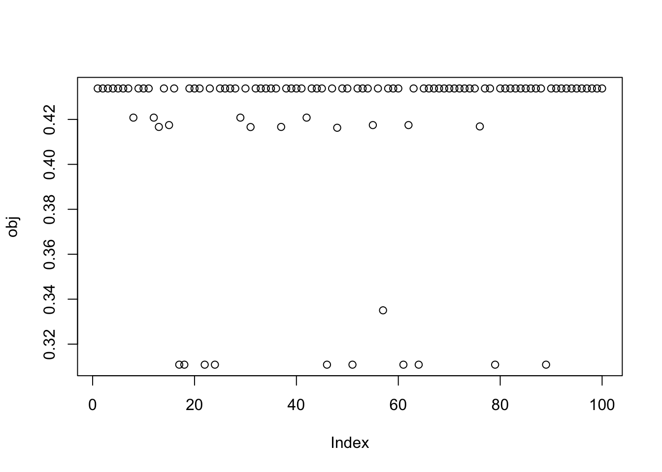
| Version | Author | Date |
|---|---|---|
| cbf04fa | Matthew Stephens | 2025-11-18 |
plot(sort(obj[obj>0.425]))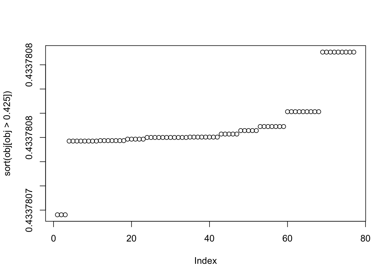
| Version | Author | Date |
|---|---|---|
| cbf04fa | Matthew Stephens | 2025-11-18 |
This is the top seed: it turns out to put all the objects in the same group! So that’s not ideal, but it makes sense that this is a solution. We either have to hope that this is not common, or find a way to avoid that solution?
seed= order(obj,decreasing=TRUE)[1]
set.seed(seed)
w = rnorm(nrow(X1))
for(i in 1:100)
  w = fastica_r1update(X1,w)
cor(L,t(X1) %*% w)
[,1]
[1,] 0.016017901
[2,] 0.032461399
[3,] 0.005764897
[4,] 0.036137004
[5,] -0.022285775
[6,] -0.004294655
[7,] -0.006035731
[8,] 0.010988125
[9,] -0.030410798plot(t(X1) %*% w)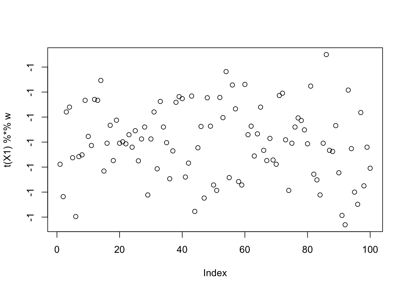
| Version | Author | Date |
|---|---|---|
| cbf04fa | Matthew Stephens | 2025-11-18 |
This is the 10th biggest seed: it finds one of the groups.
seed= order(obj,decreasing=TRUE)[10]
set.seed(seed)
w = rnorm(nrow(X1))
for(i in 1:100)
  w = fastica_r1update(X1,w)
cor(L,t(X1) %*% w)
[,1]
[1,] 1.278403e-08
[2,] 9.999998e-01
[3,] -1.415666e-07
[4,] 6.888338e-08
[5,] 6.250004e-02
[6,] 6.250003e-02
[7,] -6.250002e-02
[8,] 9.378755e-09
[9,] -6.249984e-02This is the 19th biggest seed: it finds another of the groups.
seed= order(obj,decreasing=TRUE)[19]
set.seed(seed)
w = rnorm(nrow(X1))
for(i in 1:100)
  w = fastica_r1update(X1,w)
cor(L,t(X1) %*% w)
[,1]
[1,] -6.249994e-02
[2,] -1.313417e-07
[3,] 9.999997e-01
[4,] 6.249995e-02
[5,] -1.790321e-07
[6,] -7.596810e-08
[7,] 1.875000e-01
[8,] 1.875001e-01
[9,] -2.500001e-01This is the smallest seed: it also finds a binary group.
seed= order(obj,decreasing=TRUE)[100]
set.seed(seed)
w = rnorm(nrow(X1))
for(i in 1:100)
  w = fastica_r1update(X1,w)
cor(L,t(X1) %*% w)
[,1]
[1,] 0.0002492304
[2,] -0.9999997059
[3,] 0.0001729523
[4,] -0.0001296219
[5,] -0.0624890613
[6,] -0.0625796239
[7,] 0.0624271317
[8,] 0.0001250855
[9,] 0.0624629152plot(t(X1) %*% w)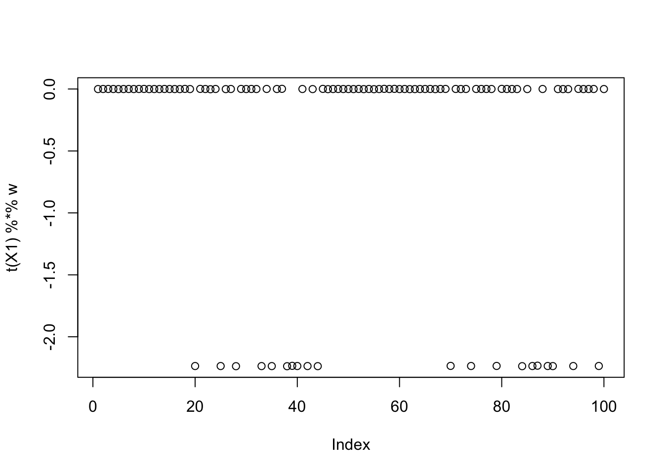
| Version | Author | Date |
|---|---|---|
| cbf04fa | Matthew Stephens | 2025-11-18 |
Four non-overlapping groups
Here I look at 4 equal non-overlapping groups. I’m interested in whether it converges to a single group or a combination of groups. It turns out that the majority of random starts converge to a combination of 2 groups, which is very different behavior than above. It gets me wondering whether this is because i) the non-overlapping situation, or ii) the symmetry created by the fact there are only 4 groups (2 vs 2).
set.seed(1)
n = 100
p = 1000
L = matrix(0,nrow=n,ncol=4)
L[1:25,1] = 1
L[26:50,2] = 1
L[51:75,3]  = 1
L[76:100,4] = 1
FF = matrix(rnorm(p*4),nrow=p)
X = L %*% t(FF) + rnorm(n*p,0,0.01)
image(X%*% t(X))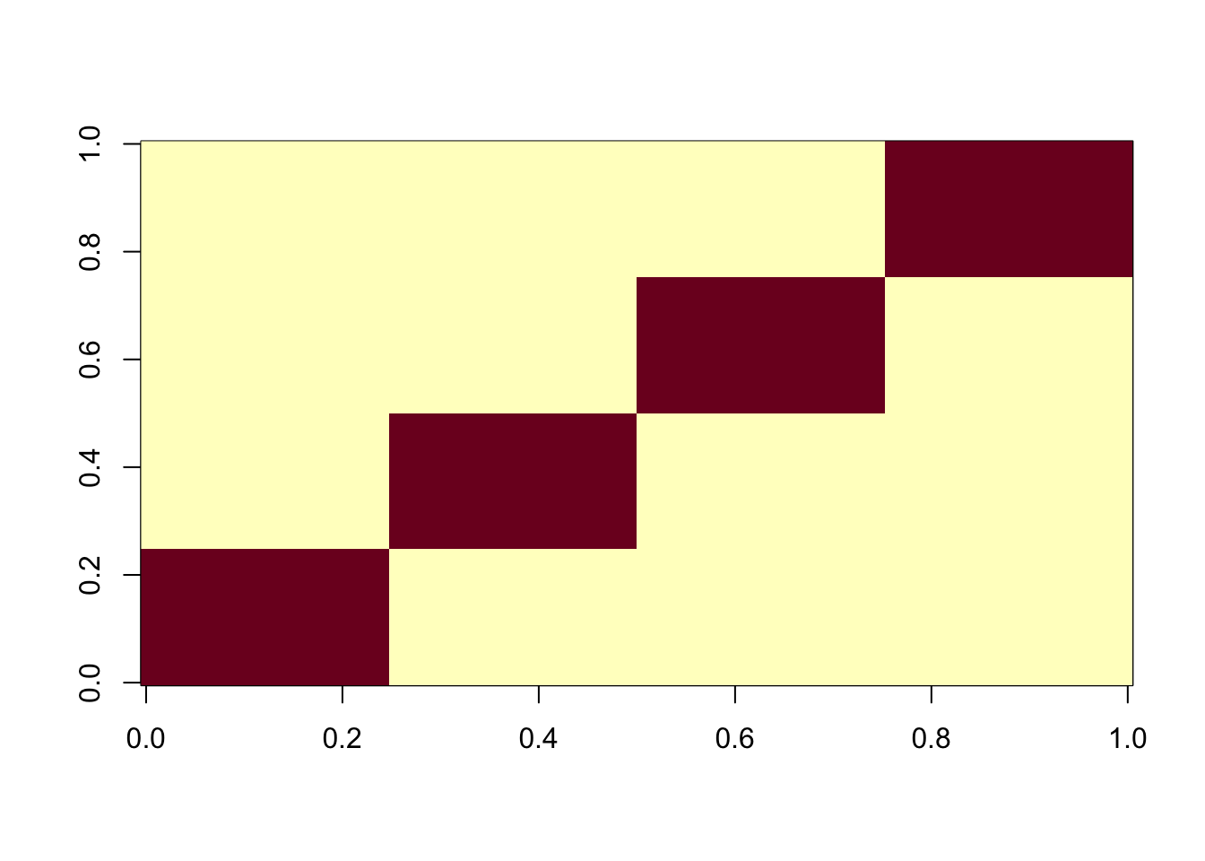
| Version | Author | Date |
|---|---|---|
| cbf04fa | Matthew Stephens | 2025-11-18 |
X1 = preprocess(X,n.comp=4)
X1 = rbind(rep(1,ncol(X1)), X1)
Here I try with 100 random starts - all of them reach an objective corresponding to a binary group. The highest objectives correspond to a single group (the trivial solution). Then the next highest correspond to single groups. The lowest correspond to combinations of 2 groups.
obj = rep(0,100)
Lhat = matrix(nrow=100,ncol=n)
for(seed in 1:100){
  set.seed(seed)
  w = rnorm(nrow(X1))
  for(i in 1:100)
    w = fastica_r1update(X1,w)
  obj[seed] = compute_objective(X1,w)
  Lhat[seed,] = t(X1) %*% w
}
plot(sort(obj))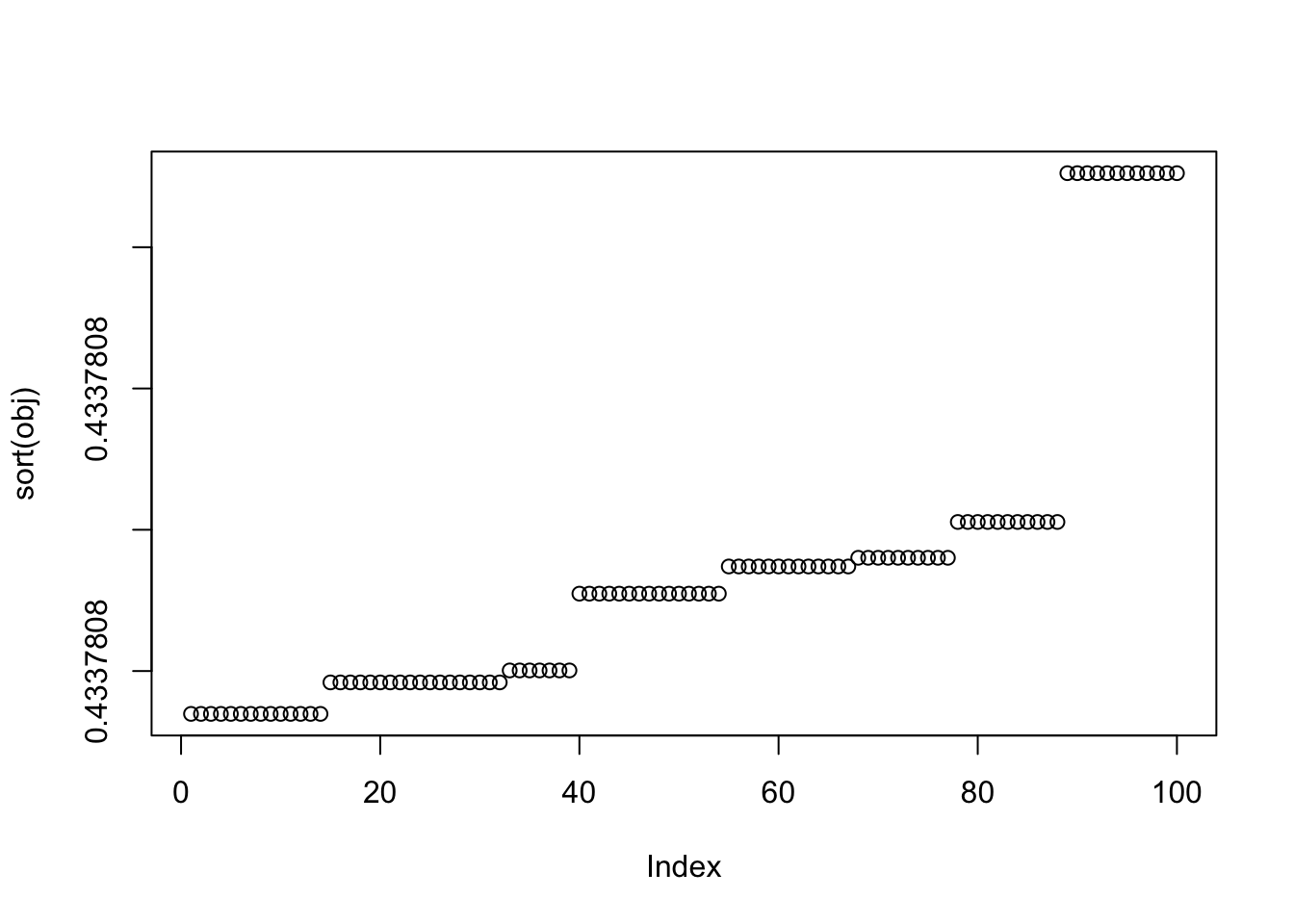
| Version | Author | Date |
|---|---|---|
| cbf04fa | Matthew Stephens | 2025-11-18 |
image(Lhat[order(obj,decreasing=TRUE),])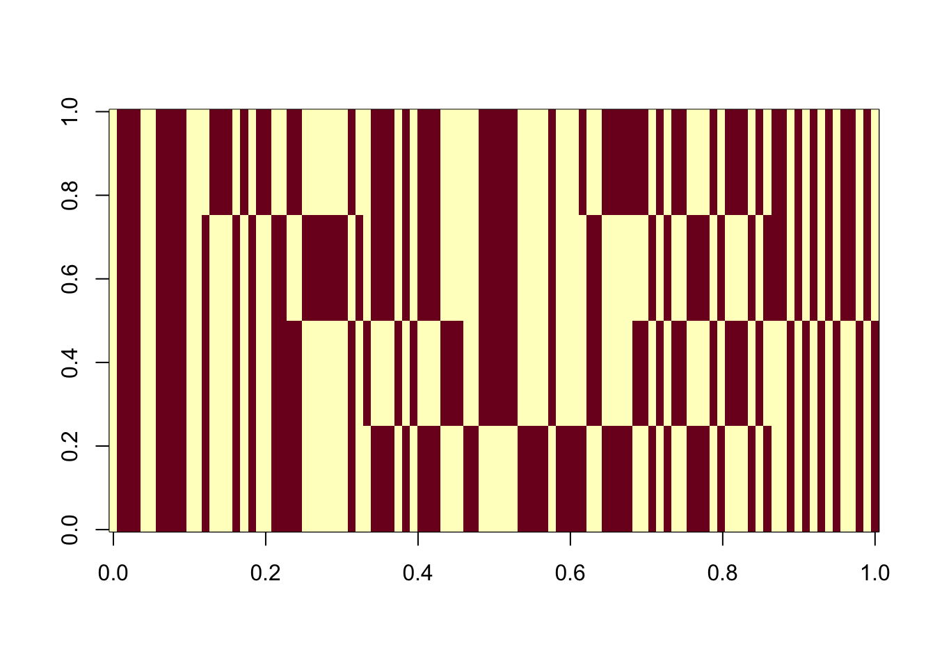
| Version | Author | Date |
|---|---|---|
| cbf04fa | Matthew Stephens | 2025-11-18 |
Here’s the results for the smallest objective for illustration:
seed= order(obj,decreasing=FALSE)[1]
set.seed(seed)
w = rnorm(nrow(X1))
for(i in 1:100)
  w = fastica_r1update(X1,w)
plot(t(X1) %*% w)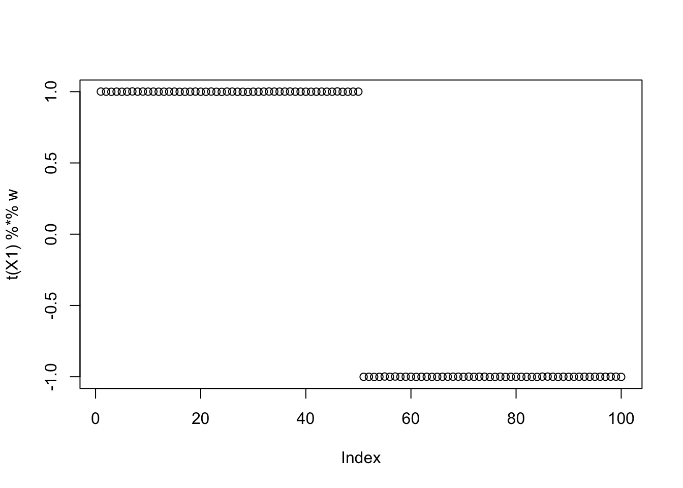
| Version | Author | Date |
|---|---|---|
| cbf04fa | Matthew Stephens | 2025-11-18 |
Nine non-overlapping groups
Here I look at 9 equal non-overlapping groups.
Start by creating L to be a binary matrix with 9 columns, 25*9 rows, and a single 1 in each row.
set.seed(1)
n = 225
p = 1000
L = matrix(0,nrow=n,ncol=9)
for(i in 1:9){L[((i-1)*25+1):(i*25),i] = 1}
FF = matrix(rnorm(p*9),nrow=p)
X = L %*% t(FF) + rnorm(n*p,0,0.01)
image(X%*% t(X))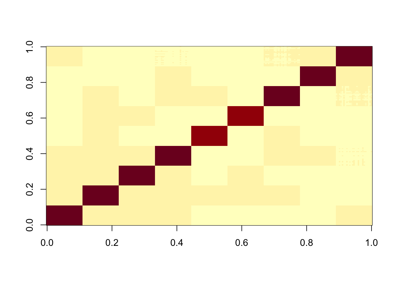
| Version | Author | Date |
|---|---|---|
| cbf04fa | Matthew Stephens | 2025-11-18 |
X1 = preprocess(X,n.comp=10)
X1 = rbind(rep(1,ncol(X1)), X1)
Here I try with 100 random starts - all of them reach an objective corresponding to a binary group, but now it finds both maxima and minima. The highest and lowest objectives correspond to single groups.
obj = rep(0,100)
Lhat = matrix(nrow=100,ncol=n)
for(seed in 1:100){
  set.seed(seed)
  w = rnorm(nrow(X1))
  for(i in 1:100)
    w = fastica_r1update(X1,w)
  obj[seed] = compute_objective(X1,w)
  Lhat[seed,] = t(X1) %*% w
}
plot(sort(obj))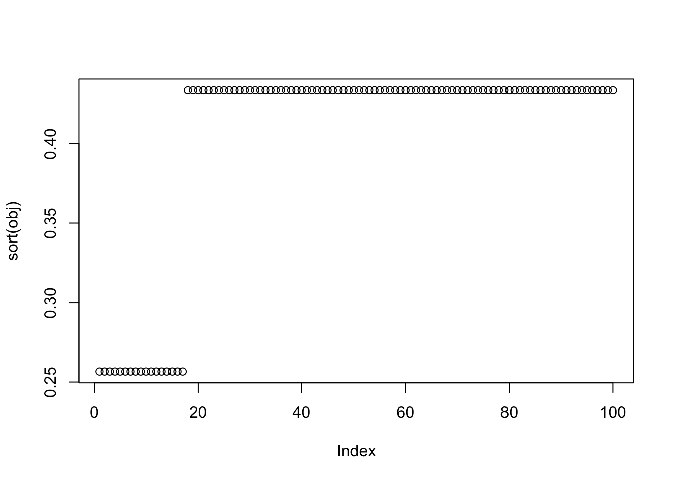
| Version | Author | Date |
|---|---|---|
| cbf04fa | Matthew Stephens | 2025-11-18 |
plot(sort(obj[obj>0.4]))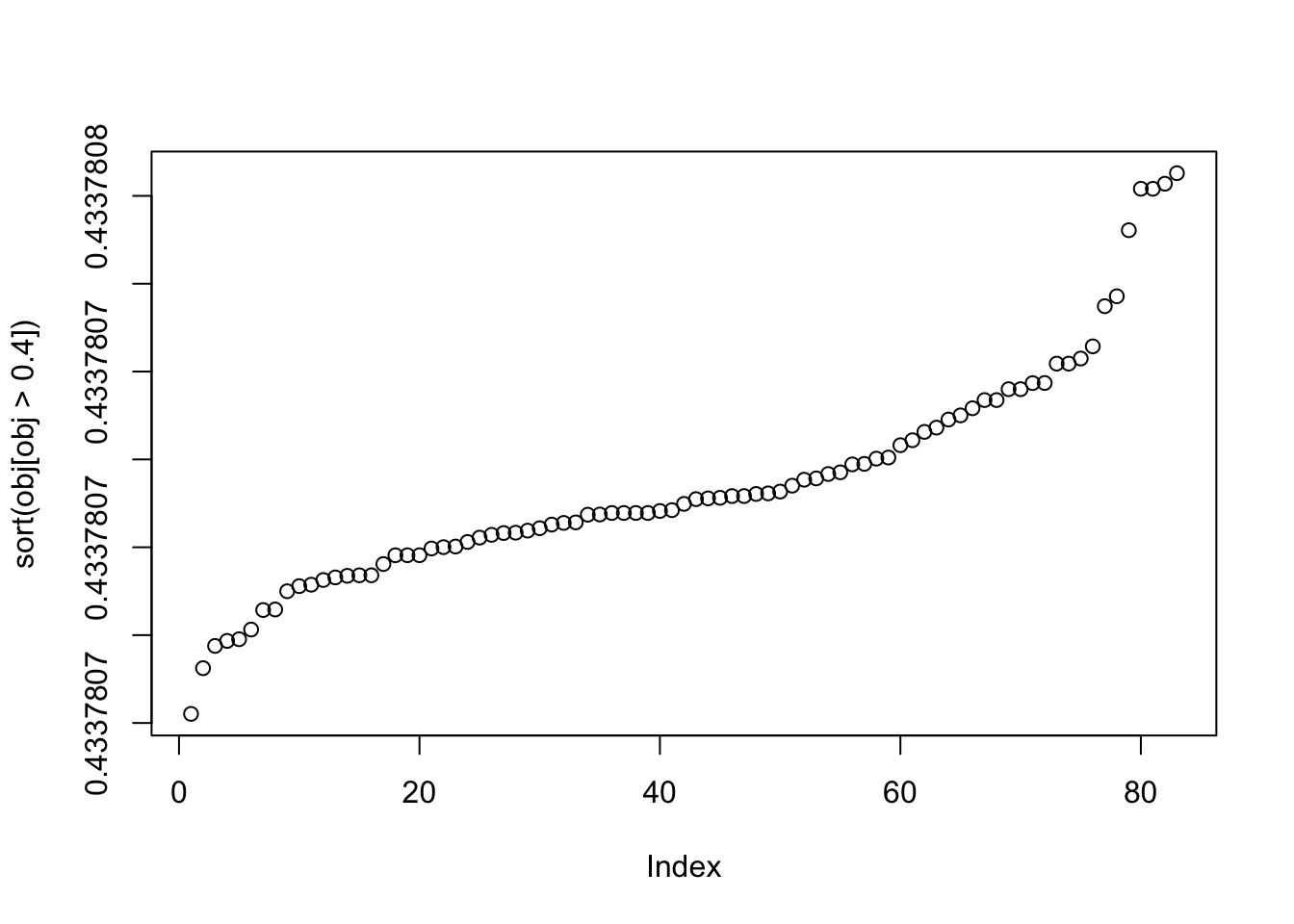
| Version | Author | Date |
|---|---|---|
| cbf04fa | Matthew Stephens | 2025-11-18 |
image(Lhat[order(obj,decreasing=TRUE),])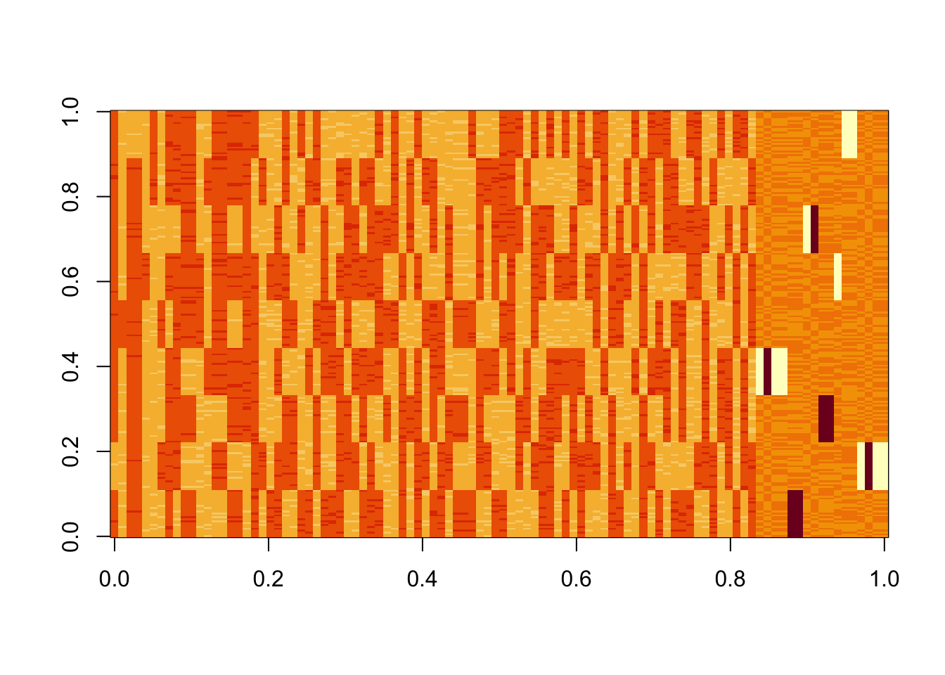
| Version | Author | Date |
|---|---|---|
| cbf04fa | Matthew Stephens | 2025-11-18 |
Bifurcating Tree simulations
Here is a simple tree-based simulations; it’s a 4-leaf tree with two bifurcating branches.
# set up L to be a tree with 4 tips and 7 branches (including top shared branch)
set.seed(1)
n = 100
p = 1000
L = matrix(0,nrow=n,ncol=6)
L[1:50,1] = 1 #top split L
L[51:100,2] = 1 # top split R
L[1:25,3]  = 1
L[26:50,4] = 1
L[51:75,5] = 1
L[76:100,6] = 1
FF = matrix(rnorm(p*6),nrow=p)
X = L %*% t(FF) + rnorm(n*p,0,0.01)
image(X%*% t(X))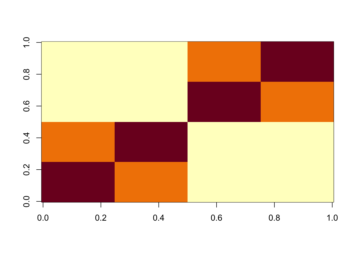
| Version | Author | Date |
|---|---|---|
| cbf04fa | Matthew Stephens | 2025-11-18 |
X1 = preprocess(X)
X1 = rbind(rep(1,ncol(X1)), X1)
Here I try with 100 random starts - most of them seem to reach an objective corresponding to a binary group, but now it finds both maxima and minima. The highest objectives are the trivial solutions; the next highest are the top split in the tree; the next highest are single branches. The lowest objectives are a bit messy so I’ll look at them in more detail next.
obj = rep(0,100)
Lhat = matrix(nrow=100,ncol=n)
for(seed in 1:100){
  set.seed(seed)
  w = rnorm(nrow(X1))
  for(i in 1:100)
    w = fastica_r1update(X1,w)
  obj[seed] = compute_objective(X1,w)
  Lhat[seed,] = t(X1) %*% w
}
plot(sort(obj))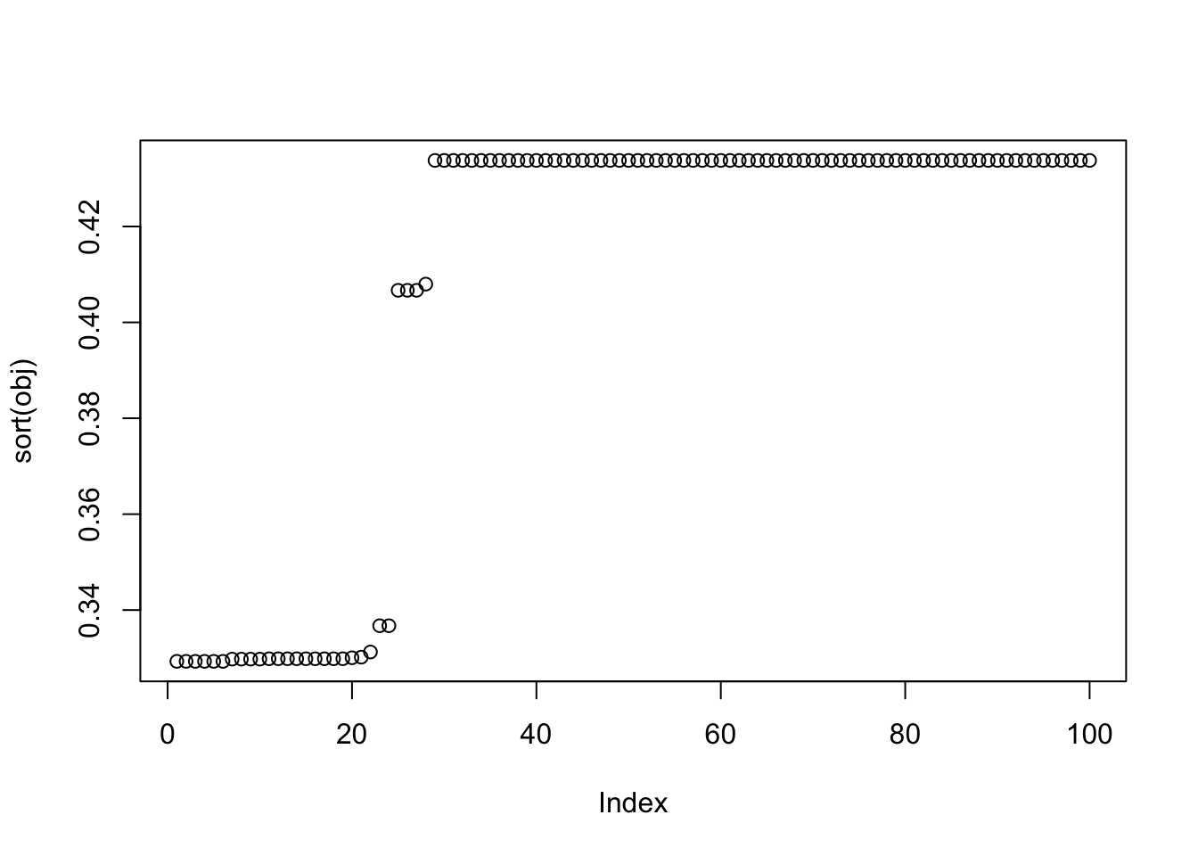
| Version | Author | Date |
|---|---|---|
| cbf04fa | Matthew Stephens | 2025-11-18 |
plot(sort(obj[obj>0.43]))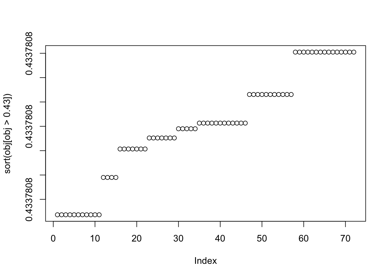
| Version | Author | Date |
|---|---|---|
| cbf04fa | Matthew Stephens | 2025-11-18 |
image(Lhat[order(obj,decreasing=TRUE),])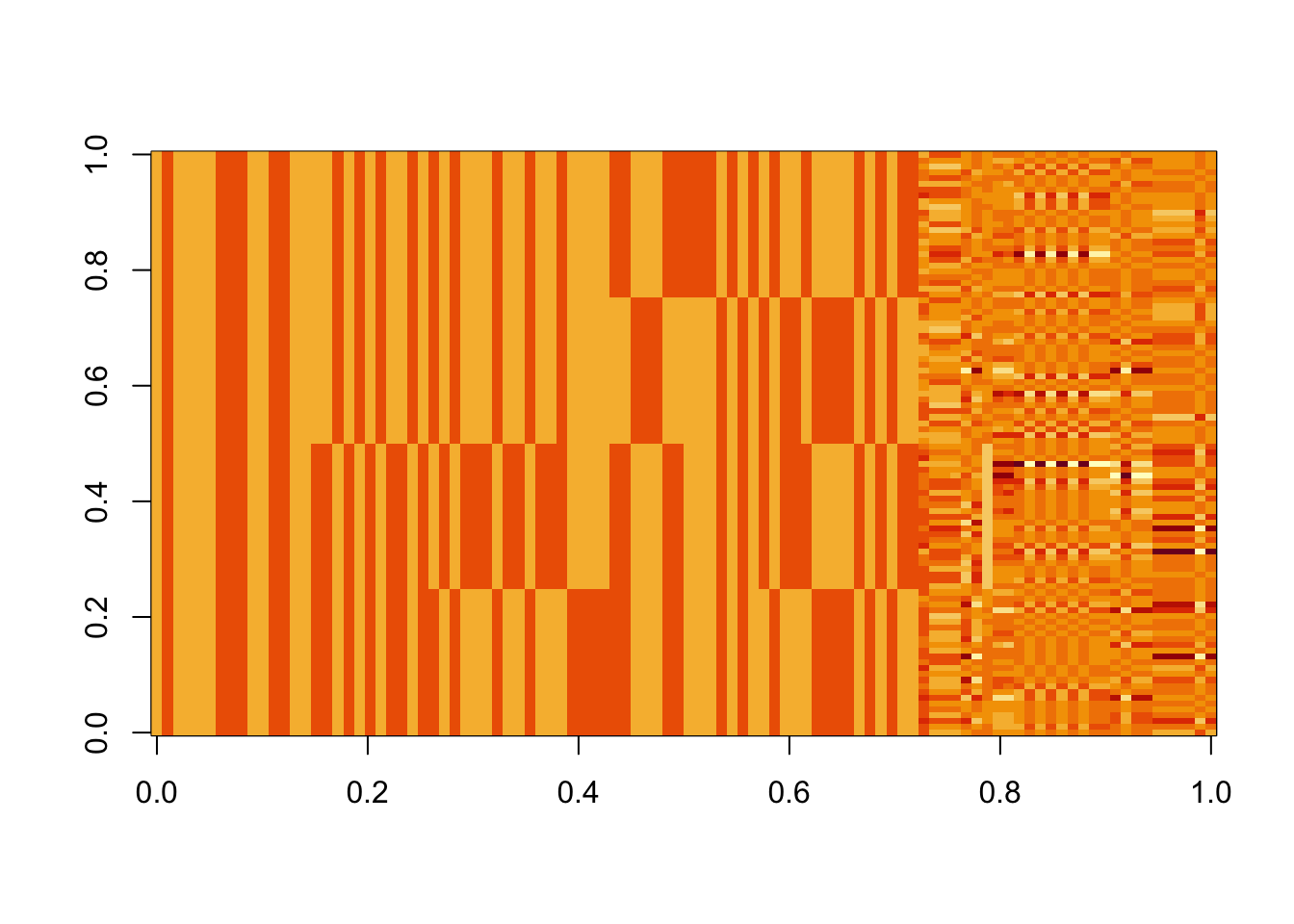
| Version | Author | Date |
|---|---|---|
| cbf04fa | Matthew Stephens | 2025-11-18 |
Here is the smallest seed: it does not actually correspond to a binary solution.
seed= order(obj,decreasing=FALSE)[1]
set.seed(seed)
w = rnorm(nrow(X1))
for(i in 1:100)
  w = fastica_r1update(X1,w)
plot(t(X1) %*% w)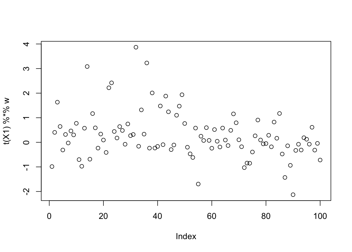
| Version | Author | Date |
|---|---|---|
| cbf04fa | Matthew Stephens | 2025-11-18 |
cor(L,t(X1) %*% w) [,1]
[1,] 0.38799777
[2,] -0.38799777
[3,] 0.09839565
[4,] 0.34962558
[5,] -0.21006434
[6,] -0.23795689Here I try preprocessing to fewer PCs to reduce the noise.
X1 = preprocess(X,n.comp=4)
X1 = rbind(rep(1,ncol(X1)), X1)
Run 100 seeds: we lose the noisy minimizing solutions.
obj = rep(0,100)
Lhat = matrix(nrow=100,ncol=n)
for(seed in 1:100){
  set.seed(seed)
  w = rnorm(nrow(X1))
  for(i in 1:100)
    w = fastica_r1update(X1,w)
  obj[seed] = compute_objective(X1,w)
  Lhat[seed,] = t(X1) %*% w
}
plot(sort(obj))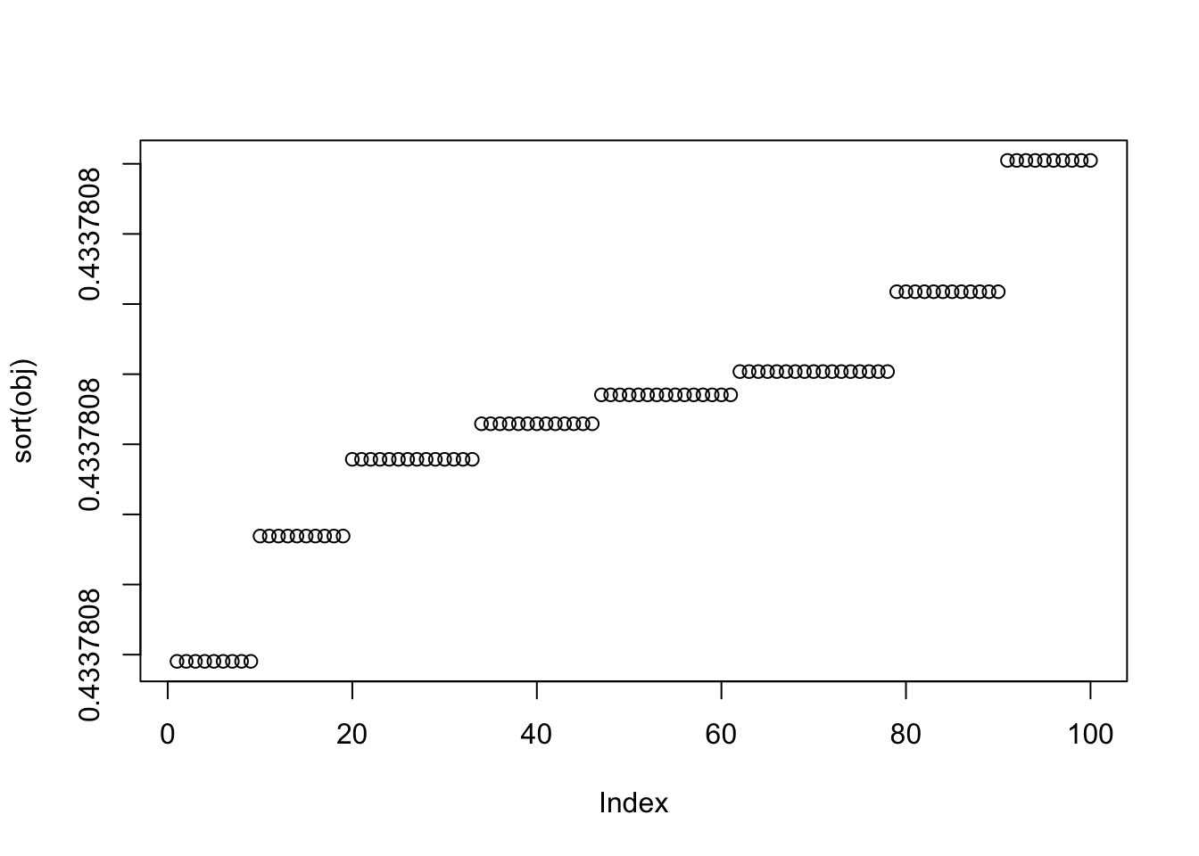
| Version | Author | Date |
|---|---|---|
| cbf04fa | Matthew Stephens | 2025-11-18 |
image(Lhat[order(obj,decreasing=TRUE),])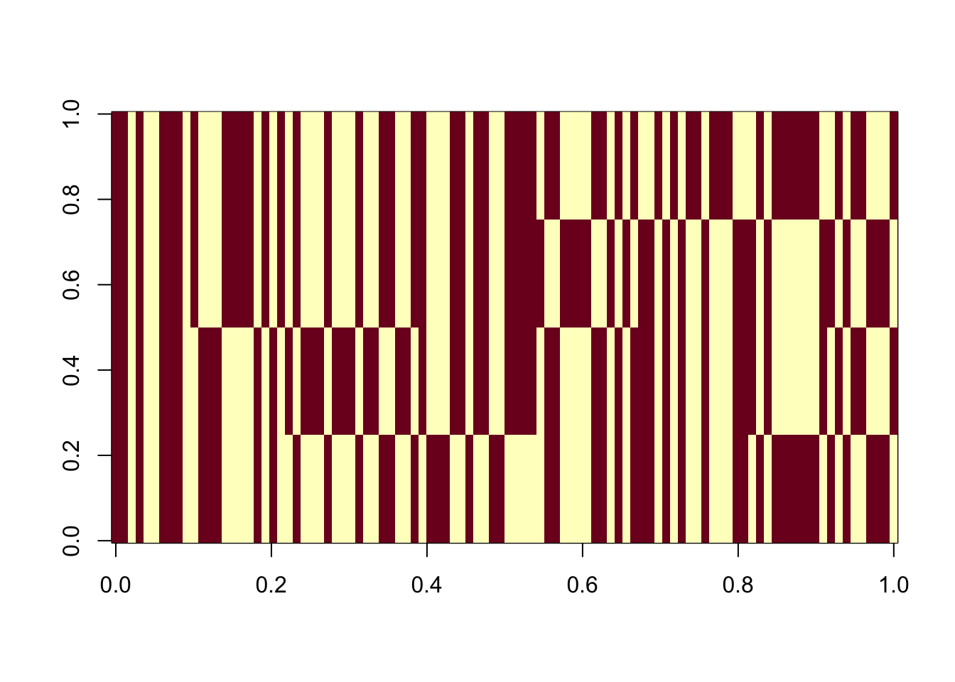
| Version | Author | Date |
|---|---|---|
| cbf04fa | Matthew Stephens | 2025-11-18 |
Adding noise
In the above the preprocessing was mostly done with adding minimal noise (ie as if we knew the true number of components). I found that performance of ICA was much degraded, even in simple examples, by more noise. This section was added to document this.
9 group simulations
To illustrate, I use the simple 9 group simulation with 20 members each. But in my preprocessing I use 20 components rather than the 10 I used above.
K=9
p = 1000
n = 100
set.seed(1)
L = matrix(0,nrow=n,ncol=K)
for(i in 1:K){L[sample(1:n,20),i]=1}
FF = matrix(rnorm(p*K), nrow = p, ncol=K)

X = L %*% t(FF) + rnorm(n*p,0,0.01)
plot(X %*% FF[,1])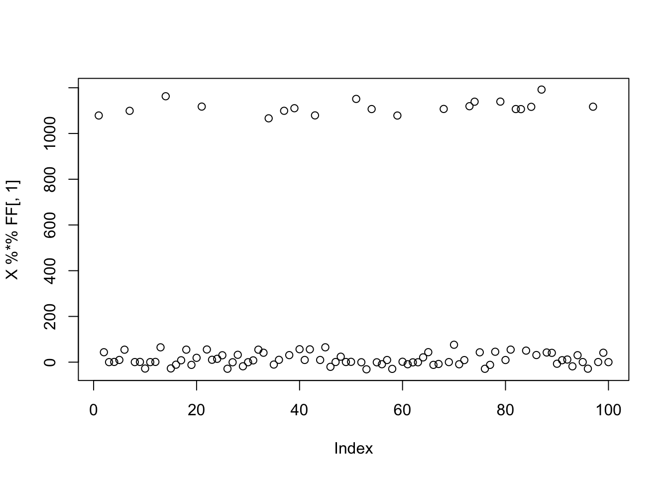
X1 = preprocess(X,n.comp=20)
X1 = rbind(rep(1,ncol(X1)), X1)
noncentered fastICA (100 random starts)
Here I try with 100 random starts - a small minority find a good group solution. Also, most of the runs seems to end up at a local minima of the objective rather than a local maximum.
obj = rep(0,100)
for(seed in 1:100){
  set.seed(seed)
  w = rnorm(nrow(X1))
  for(i in 1:100)
    w = fastica_r1update(X1,w)
  obj[seed] = compute_objective(X1,w)
}
plot(obj)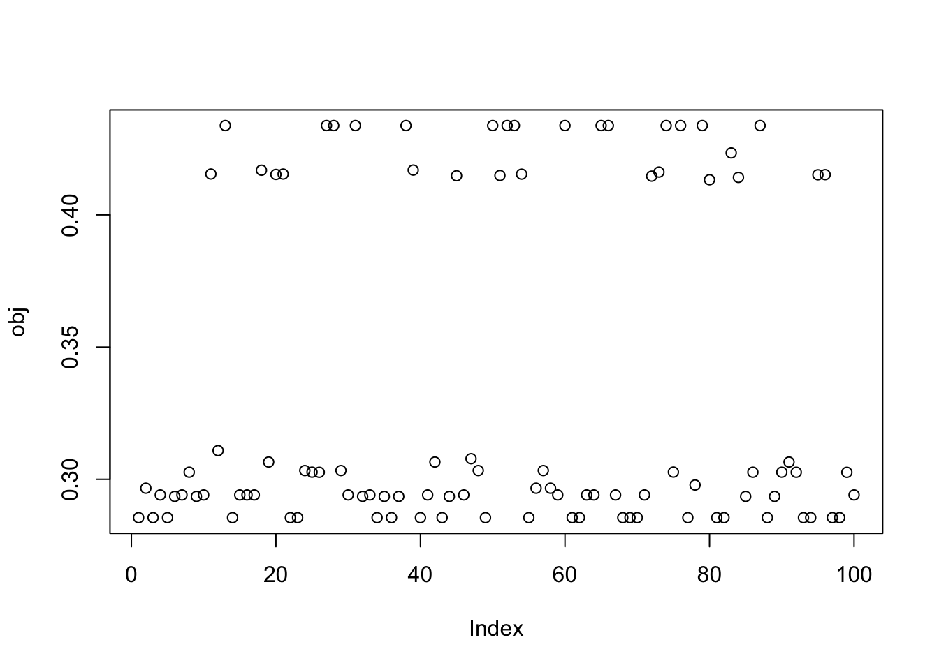
plot(sort(obj[obj>0.425]))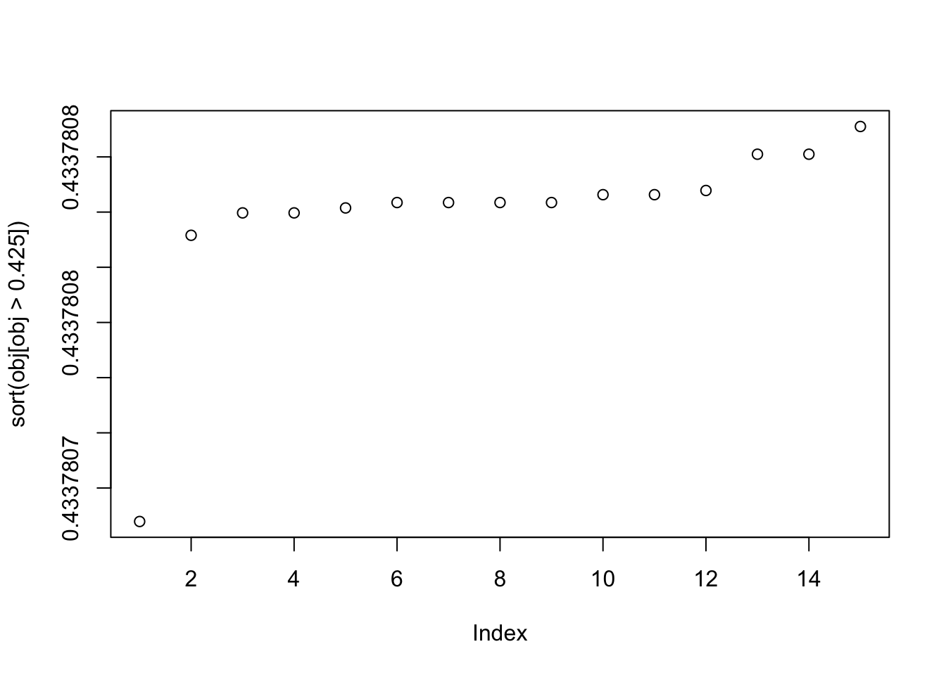
This is the bottom seed: you can see it picks out a “laplace-like” distribution, which gives a small logcosh value.
seed= order(obj,decreasing=TRUE)[100]
set.seed(seed)
w = rnorm(nrow(X1))
for(i in 1:100)
  w = fastica_r1update(X1,w)
cor(L,t(X1) %*% w)
[,1]
[1,] -0.326382613
[2,] 0.139316540
[3,] -0.287943408
[4,] -0.366600144
[5,] -0.120411055
[6,] -0.347279430
[7,] -0.293360295
[8,] 0.095506593
[9,] -0.003713107plot(t(X1) %*% w)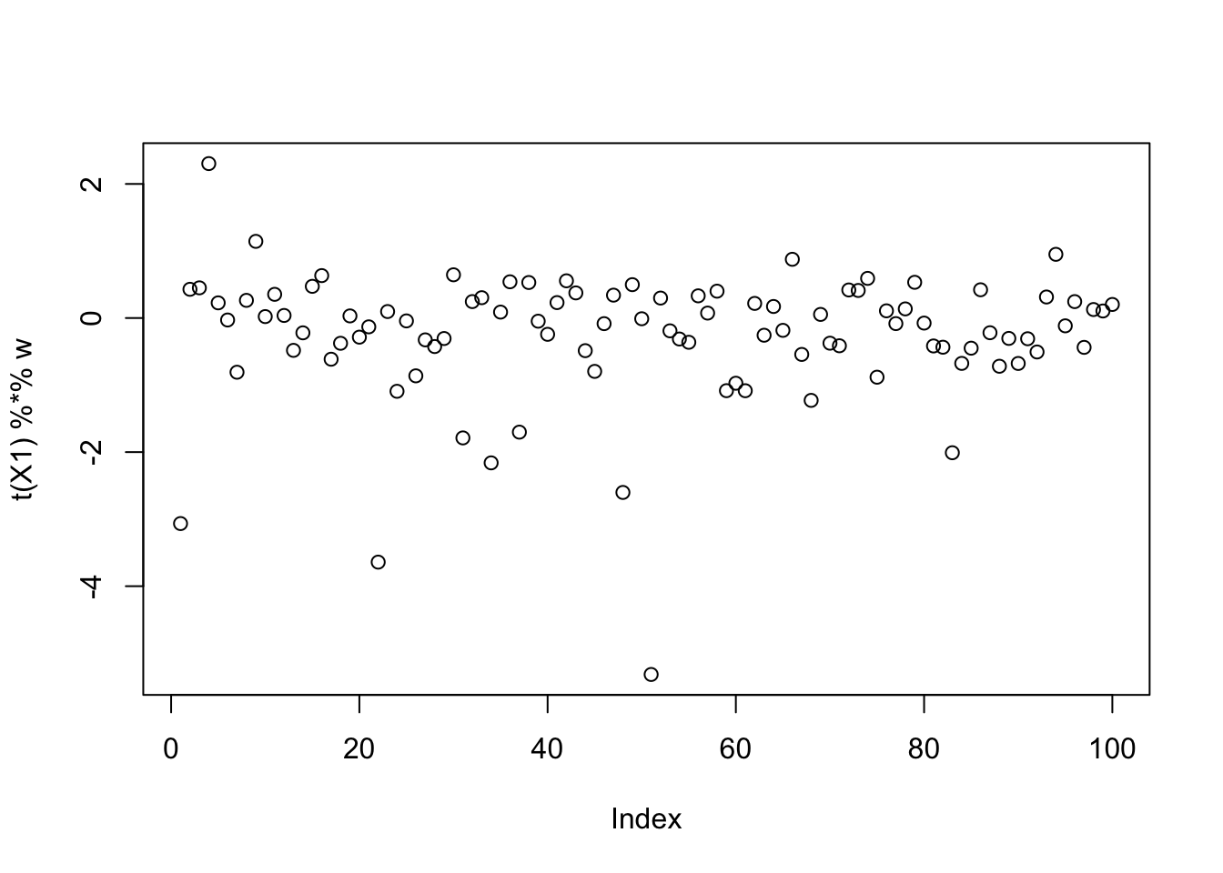
EBCD, 100 random starts
When we remove the G2 term from the fastICA updates, this is essentially the single-unit EBCD updates from Kang + Stephens. These are designed to maximize the objective, so I try those here. Now all the runs get a larger value for the objective. However, they mostly don’t seem to be quite finding the single group solutions, and indeed further investigation suggests they are finding a combination of groups.
obj = rep(0,100)
for(seed in 1:100){
  set.seed(seed)
  w = rnorm(nrow(X1))
  for(i in 1:100)
    w = fastica_r1update(X1,w,includeG2=FALSE)
  obj[seed] = compute_objective(X1,w)
}
plot(obj)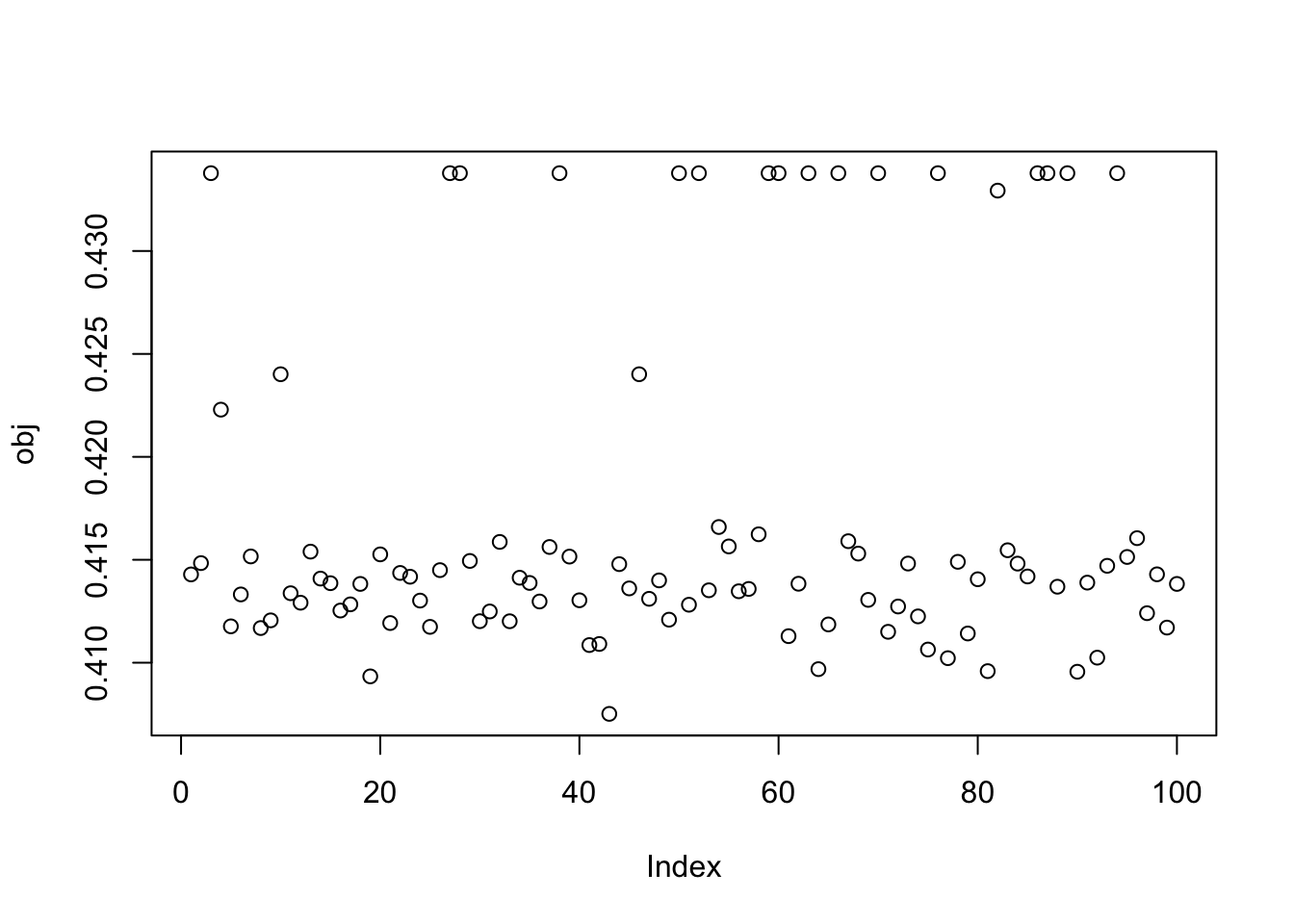
This is the bottom seed:
seed= order(obj,decreasing=TRUE)[100]
set.seed(seed)
w = rnorm(nrow(X1))
for(i in 1:100)
  w = fastica_r1update(X1,w,includeG2=FALSE)
cor(L,t(X1) %*% w)
[,1]
[1,] -0.13162305
[2,] 0.06824820
[3,] 0.25676124
[4,] 0.00623320
[5,] 0.12218955
[6,] -0.41205507
[7,] 0.11329491
[8,] 0.01312181
[9,] -0.08260268plot(t(X1) %*% w)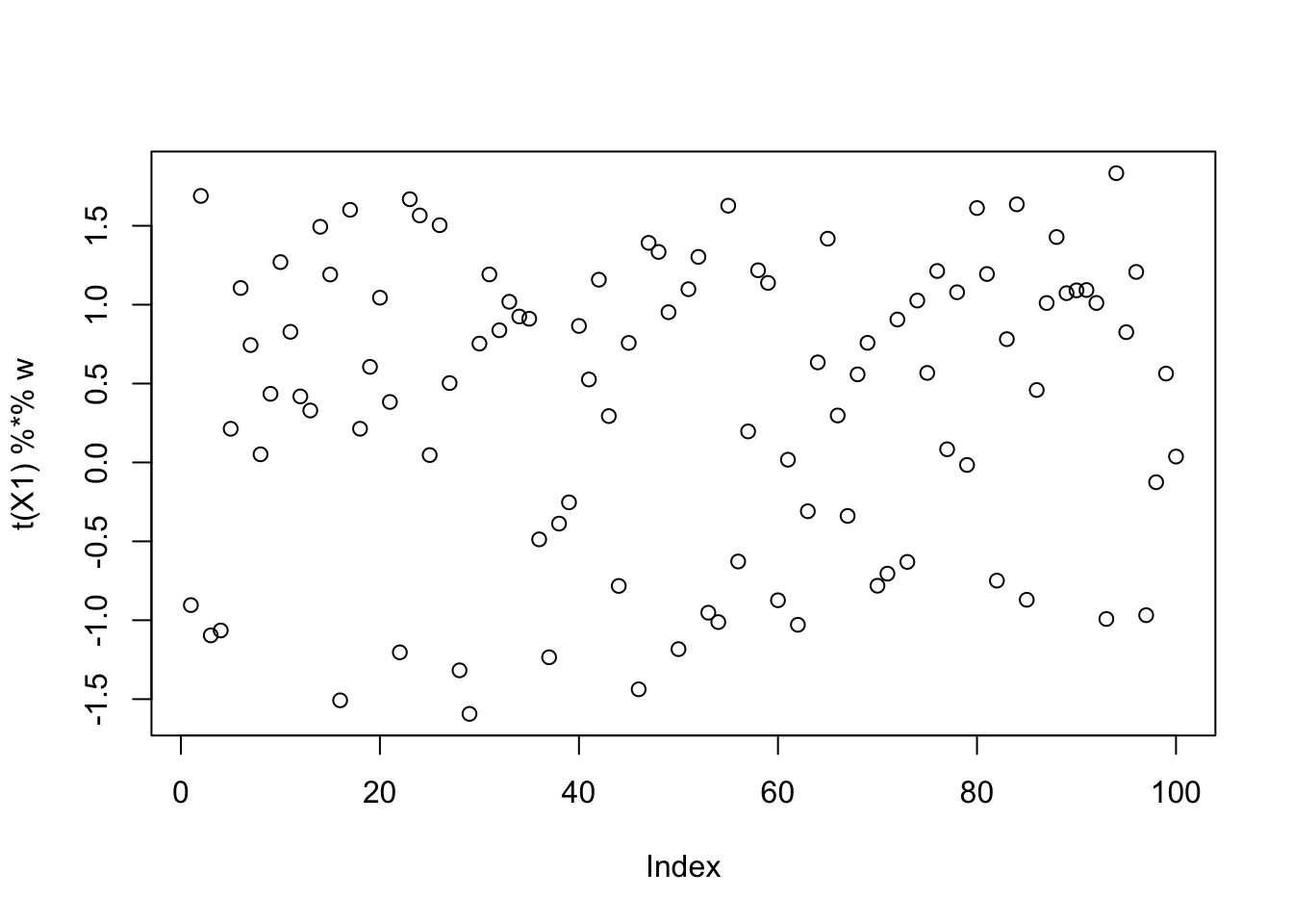
This is a middle seed
seed= order(obj,decreasing=TRUE)[50]
set.seed(seed)
w = rnorm(nrow(X1))
for(i in 1:100)
  w = fastica_r1update(X1,w,includeG2=FALSE)
cor(L,t(X1) %*% w)
[,1]
[1,] 0.22353927
[2,] -0.08237851
[3,] -0.11528183
[4,] -0.08373376
[5,] -0.12000474
[6,] 0.02493547
[7,] -0.14642010
[8,] -0.05737402
[9,] -0.04951017plot(t(X1) %*% w)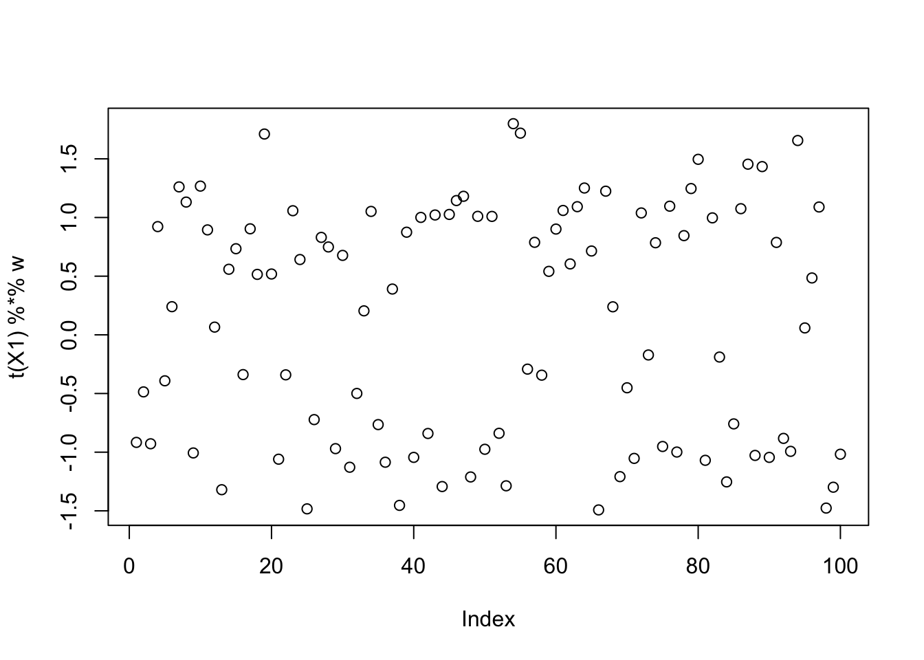
It looks like these solutions are “on their way” to binary, but not yet binary. I could try running more iterations to see if it changes, but here I add on the fastICA updates (with G2) to see what happens. That is, here I’m initializing fastICA with the EBCD results. It does not seem to change much.
obj = rep(0,100)
for(seed in 1:100){
  set.seed(seed)
  w = rnorm(nrow(X1))
  for(i in 1:100)
    w = fastica_r1update(X1,w,includeG2=FALSE)
  for(i in 1:100)
    w = fastica_r1update(X1,w,includeG2=TRUE)
  obj[seed] = compute_objective(X1,w)
}
plot(obj)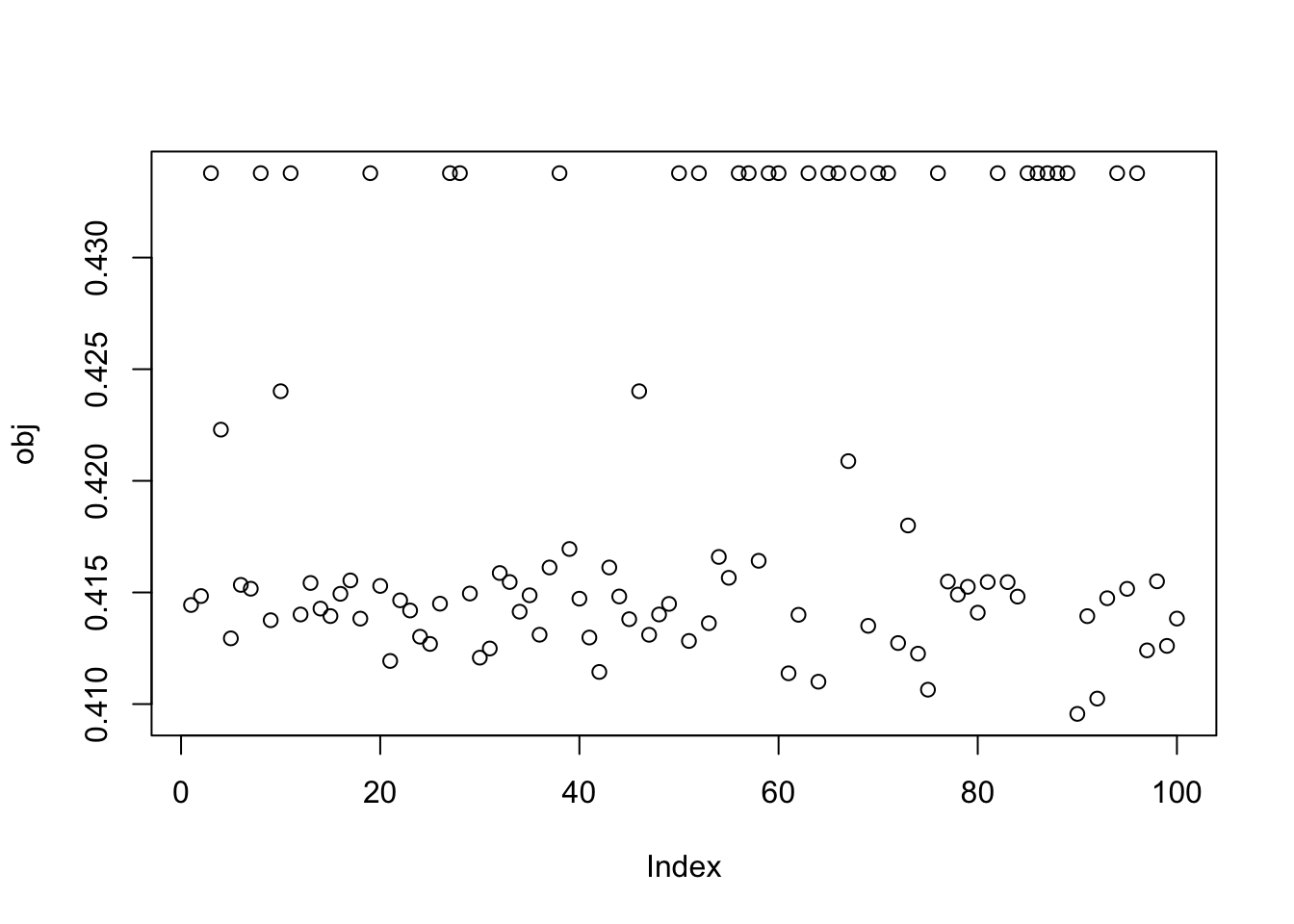
This is a middle seed
seed= order(obj,decreasing=TRUE)[50]
set.seed(seed)
w = rnorm(nrow(X1))
for(i in 1:100)
    w = fastica_r1update(X1,w,includeG2=FALSE)
for(i in 1:100)
    w = fastica_r1update(X1,w,includeG2=TRUE)
cor(L,t(X1) %*% w)
[,1]
[1,] -0.11943895
[2,] -0.13933167
[3,] -0.05794822
[4,] 0.07074235
[5,] -0.18979351
[6,] 0.18245595
[7,] -0.30135190
[8,] 0.30324477
[9,] -0.09724178plot(t(X1) %*% w)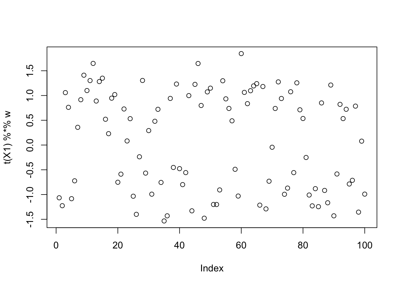
Here I try running just a couple of EBCD updates to encourage fastICA to maximize rather than minimize. It definitely helps it to find a local maximum, but a lot of the local optima are still not the single-group solutions.
obj = rep(0,100)
for(seed in 1:100){
  set.seed(seed)
  w = rnorm(nrow(X1))
  for(i in 1:2)
    w = fastica_r1update(X1,w,includeG2=FALSE)
  for(i in 1:100)
    w = fastica_r1update(X1,w,includeG2=TRUE)
  obj[seed] = compute_objective(X1,w)
}
plot(obj)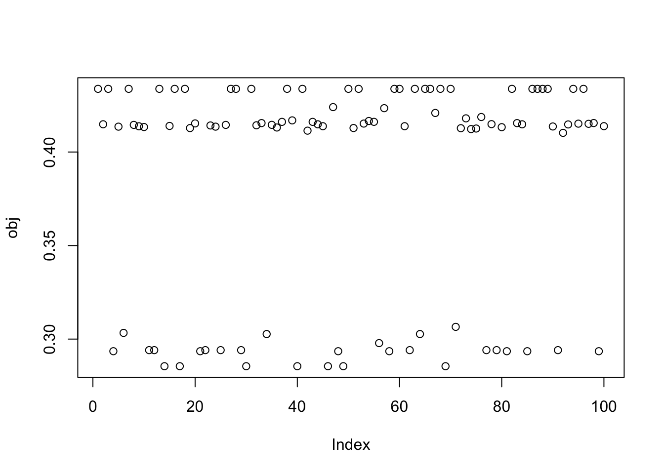
This is a middle seed again:
seed= order(obj,decreasing=TRUE)[50]
set.seed(seed)
w = rnorm(nrow(X1))
for(i in 1:2)
    w = fastica_r1update(X1,w,includeG2=FALSE)
for(i in 1:100)
    w = fastica_r1update(X1,w,includeG2=TRUE)
cor(L,t(X1) %*% w)
[,1]
[1,] 0.491974448
[2,] 0.343688283
[3,] 0.148582808
[4,] 0.253684992
[5,] -0.221511403
[6,] -0.005607077
[7,] -0.377128781
[8,] 0.052999128
[9,] -0.169368405plot(t(X1) %*% w)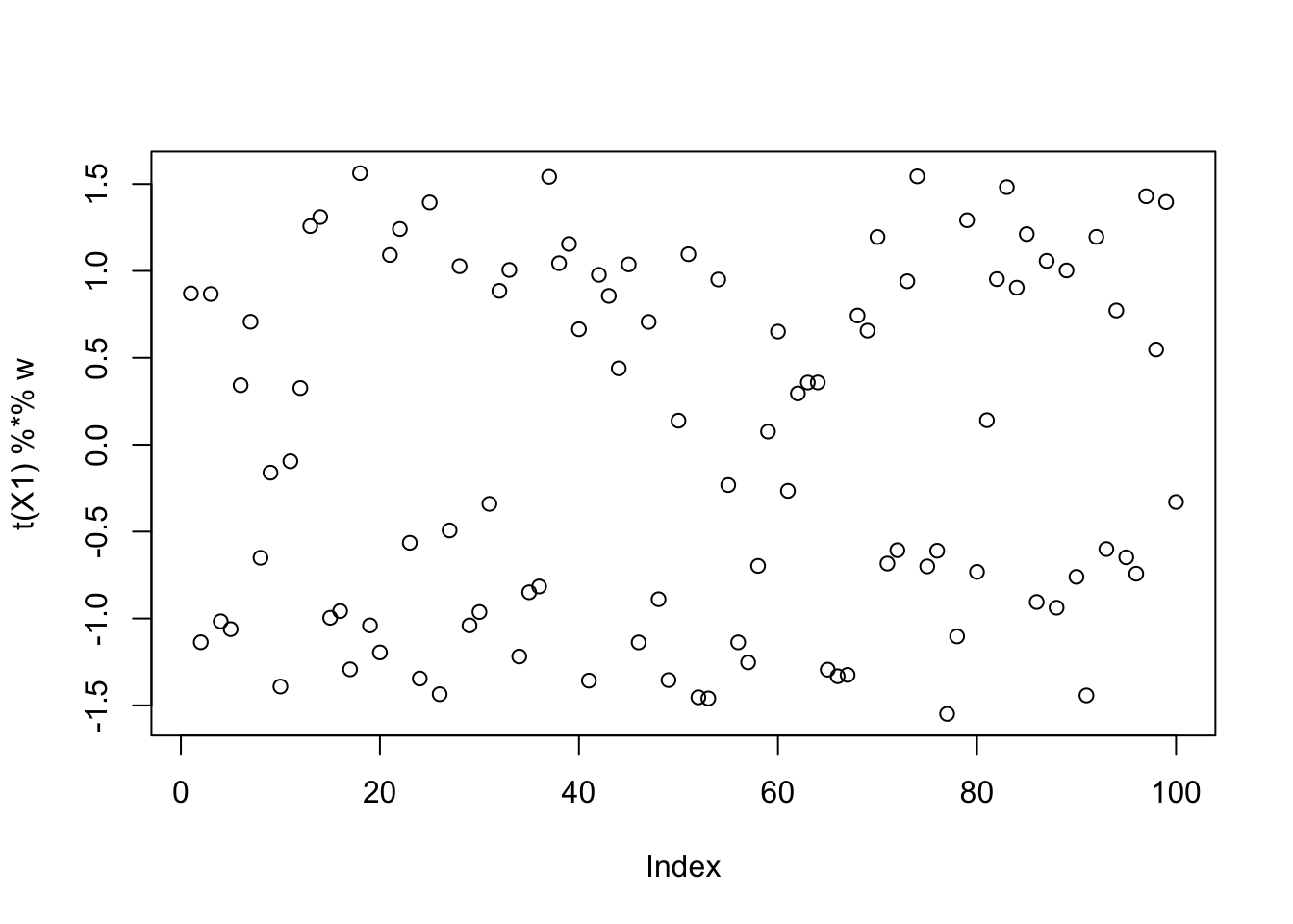
sessionInfo()R version 4.4.2 (2024-10-31)
Platform: aarch64-apple-darwin20
Running under: macOS Sequoia 15.6.1
Matrix products: default
BLAS: /Library/Frameworks/R.framework/Versions/4.4-arm64/Resources/lib/libRblas.0.dylib
LAPACK: /Library/Frameworks/R.framework/Versions/4.4-arm64/Resources/lib/libRlapack.dylib; LAPACK version 3.12.0
locale:
[1] en_US.UTF-8/en_US.UTF-8/en_US.UTF-8/C/en_US.UTF-8/en_US.UTF-8
time zone: America/Chicago
tzcode source: internal
attached base packages:
[1] stats graphics grDevices utils datasets methods base
loaded via a namespace (and not attached):
[1] vctrs_0.6.5 cli_3.6.5 knitr_1.50 rlang_1.1.6
[5] xfun_0.52 stringi_1.8.7 promises_1.3.3 jsonlite_2.0.0
[9] workflowr_1.7.1 glue_1.8.0 rprojroot_2.0.4 git2r_0.35.0
[13] htmltools_0.5.8.1 httpuv_1.6.15 sass_0.4.10 rmarkdown_2.29
[17] evaluate_1.0.4 jquerylib_0.1.4 tibble_3.3.0 fastmap_1.2.0
[21] yaml_2.3.10 lifecycle_1.0.4 whisker_0.4.1 stringr_1.5.1
[25] compiler_4.4.2 fs_1.6.6 Rcpp_1.0.14 pkgconfig_2.0.3
[29] rstudioapi_0.17.1 later_1.4.2 digest_0.6.37 R6_2.6.1
[33] pillar_1.10.2 magrittr_2.0.3 bslib_0.9.0 tools_4.4.2
[37] cachem_1.1.0