EB_subspace

Last updated: 2026-06-21

Checks: 7 0

Knit directory: misc/analysis/

This reproducible R Markdown analysis was created with workflowr (version 1.7.2). The Checks tab describes the reproducibility checks that were applied when the results were created. The Past versions tab lists the development history.

R Markdown file: up-to-date

Great! Since the R Markdown file has been committed to the Git repository, you know the exact version of the code that produced these results.

Environment: empty

Great job! The global environment was empty. Objects defined in the global environment can affect the analysis in your R Markdown file in unknown ways. For reproduciblity it’s best to always run the code in an empty environment.

Seed: set.seed(1)

The command set.seed(1) was run prior to running the code in the R Markdown file. Setting a seed ensures that any results that rely on randomness, e.g. subsampling or permutations, are reproducible.

Session information: recorded

Great job! Recording the operating system, R version, and package versions is critical for reproducibility.

Cache: none

Nice! There were no cached chunks for this analysis, so you can be confident that you successfully produced the results during this run.

File paths: relative

Great job! Using relative paths to the files within your workflowr project makes it easier to run your code on other machines.

Repository version: 4b69522

Great! You are using Git for version control. Tracking code development and connecting the code version to the results is critical for reproducibility.

The results in this page were generated with repository version 4b69522. See the Past versions tab to see a history of the changes made to the R Markdown and HTML files.

Note that you need to be careful to ensure that all relevant files for the analysis have been committed to Git prior to generating the results (you can use wflow_publish or wflow_git_commit). workflowr only checks the R Markdown file, but you know if there are other scripts or data files that it depends on. Below is the status of the Git repository when the results were generated:


Ignored files:
    Ignored:    .DS_Store
    Ignored:    .Rhistory
    Ignored:    .Rproj.user/
    Ignored:    GSE87571/
    Ignored:    analysis/.RData
    Ignored:    analysis/.Rhistory
    Ignored:    analysis/ALStruct_cache/
    Ignored:    data/.Rhistory
    Ignored:    data/methylation-data-for-matthew.rds
    Ignored:    data/pbmc/
    Ignored:    data/pbmc_purified.RData

Untracked files:
    Untracked:  .dropbox
    Untracked:  GSE41037/
    Untracked:  Icon
    Untracked:  analysis/GHstan.Rmd
    Untracked:  analysis/GTEX-cogaps.Rmd
    Untracked:  analysis/PACS.Rmd
    Untracked:  analysis/Rplot.png
    Untracked:  analysis/SPCAvRP.rmd
    Untracked:  analysis/abf_comparisons.Rmd
    Untracked:  analysis/admm_02.Rmd
    Untracked:  analysis/admm_03.Rmd
    Untracked:  analysis/bispca.Rmd
    Untracked:  analysis/cache/
    Untracked:  analysis/cholesky.Rmd
    Untracked:  analysis/compare-transformed-models.Rmd
    Untracked:  analysis/cormotif.Rmd
    Untracked:  analysis/cp_ash.Rmd
    Untracked:  analysis/eQTL.perm.rand.pdf
    Untracked:  analysis/eb_power2.Rmd
    Untracked:  analysis/eb_prepilot.Rmd
    Untracked:  analysis/eb_var.Rmd
    Untracked:  analysis/ebpmf1.Rmd
    Untracked:  analysis/ebpmf_sla_text.Rmd
    Untracked:  analysis/ebspca_sims.Rmd
    Untracked:  analysis/explore_psvd.Rmd
    Untracked:  analysis/fa_check_identify.Rmd
    Untracked:  analysis/fa_iterative.Rmd
    Untracked:  analysis/fastica_heated.Rmd
    Untracked:  analysis/flash_cov_overlapping_groups_init.Rmd
    Untracked:  analysis/flash_test_tree.Rmd
    Untracked:  analysis/flashier_newgroups.Rmd
    Untracked:  analysis/flashier_nmf_triples.Rmd
    Untracked:  analysis/flashier_pbmc.Rmd
    Untracked:  analysis/flashier_snn_shifted_prior.Rmd
    Untracked:  analysis/greedy_ebpmf_exploration_00.Rmd
    Untracked:  analysis/ieQTL.perm.rand.pdf
    Untracked:  analysis/lasso_em_03.Rmd
    Untracked:  analysis/m6amash.Rmd
    Untracked:  analysis/mash_bhat_z.Rmd
    Untracked:  analysis/mash_ieqtl_permutations.Rmd
    Untracked:  analysis/matrix_beta.Rmd
    Untracked:  analysis/meth_flash_01.Rmd
    Untracked:  analysis/methylation_example.Rmd
    Untracked:  analysis/mixsqp.Rmd
    Untracked:  analysis/mr.ash_lasso_init.Rmd
    Untracked:  analysis/mr.mash.test.Rmd
    Untracked:  analysis/mr_ash_modular.Rmd
    Untracked:  analysis/mr_ash_parameterization.Rmd
    Untracked:  analysis/mr_ash_ridge.Rmd
    Untracked:  analysis/mv_gaussian_message_passing.Rmd
    Untracked:  analysis/nejm.Rmd
    Untracked:  analysis/nmf_bg.Rmd
    Untracked:  analysis/nonneg_underapprox.Rmd
    Untracked:  analysis/normal_conditional_on_r2.Rmd
    Untracked:  analysis/normalize.Rmd
    Untracked:  analysis/pbmc.Rmd
    Untracked:  analysis/pca_binary_weighted.Rmd
    Untracked:  analysis/pca_l1.Rmd
    Untracked:  analysis/poisson_nmf_approx.Rmd
    Untracked:  analysis/poisson_shrink.Rmd
    Untracked:  analysis/poisson_transform.Rmd
    Untracked:  analysis/qrnotes.txt
    Untracked:  analysis/ridge_iterative_02.Rmd
    Untracked:  analysis/ridge_iterative_splitting.Rmd
    Untracked:  analysis/samps/
    Untracked:  analysis/sc_bimodal.Rmd
    Untracked:  analysis/shrinkage_comparisons_changepoints.Rmd
    Untracked:  analysis/susie_cov.Rmd
    Untracked:  analysis/susie_en.Rmd
    Untracked:  analysis/susie_z_investigate.Rmd
    Untracked:  analysis/svd-timing.Rmd
    Untracked:  analysis/temp.RDS
    Untracked:  analysis/temp.Rmd
    Untracked:  analysis/test-figure/
    Untracked:  analysis/test.Rmd
    Untracked:  analysis/test.Rpres
    Untracked:  analysis/test.md
    Untracked:  analysis/test_qr.R
    Untracked:  analysis/test_sparse.Rmd
    Untracked:  analysis/tree_dist_top_eigenvector.Rmd
    Untracked:  analysis/z.txt
    Untracked:  code/coordinate_descent_symNMF.R
    Untracked:  code/multivariate_testfuncs.R
    Untracked:  code/rqb.hacked.R
    Untracked:  data/4matthew/
    Untracked:  data/4matthew2/
    Untracked:  data/E-MTAB-2805.processed.1/
    Untracked:  data/ENSG00000156738.Sim_Y2.RDS
    Untracked:  data/GDS5363_full.soft.gz
    Untracked:  data/GSE41265_allGenesTPM.txt
    Untracked:  data/Muscle_Skeletal.ACTN3.pm1Mb.RDS
    Untracked:  data/P.rds
    Untracked:  data/Thyroid.FMO2.pm1Mb.RDS
    Untracked:  data/bmass.HaemgenRBC2016.MAF01.Vs2.MergedDataSources.200kRanSubset.ChrBPMAFMarkerZScores.vs1.txt.gz
    Untracked:  data/bmass.HaemgenRBC2016.Vs2.NewSNPs.ZScores.hclust.vs1.txt
    Untracked:  data/bmass.HaemgenRBC2016.Vs2.PreviousSNPs.ZScores.hclust.vs1.txt
    Untracked:  data/eb_prepilot/
    Untracked:  data/finemap_data/fmo2.sim/b.txt
    Untracked:  data/finemap_data/fmo2.sim/dap_out.txt
    Untracked:  data/finemap_data/fmo2.sim/dap_out2.txt
    Untracked:  data/finemap_data/fmo2.sim/dap_out2_snp.txt
    Untracked:  data/finemap_data/fmo2.sim/dap_out_snp.txt
    Untracked:  data/finemap_data/fmo2.sim/data
    Untracked:  data/finemap_data/fmo2.sim/fmo2.sim.config
    Untracked:  data/finemap_data/fmo2.sim/fmo2.sim.k
    Untracked:  data/finemap_data/fmo2.sim/fmo2.sim.k4.config
    Untracked:  data/finemap_data/fmo2.sim/fmo2.sim.k4.snp
    Untracked:  data/finemap_data/fmo2.sim/fmo2.sim.ld
    Untracked:  data/finemap_data/fmo2.sim/fmo2.sim.snp
    Untracked:  data/finemap_data/fmo2.sim/fmo2.sim.z
    Untracked:  data/finemap_data/fmo2.sim/pos.txt
    Untracked:  data/logm.csv
    Untracked:  data/m.cd.RDS
    Untracked:  data/m.cdu.old.RDS
    Untracked:  data/m.new.cd.RDS
    Untracked:  data/m.old.cd.RDS
    Untracked:  data/mainbib.bib.old
    Untracked:  data/mat.csv
    Untracked:  data/mat.txt
    Untracked:  data/mat_new.csv
    Untracked:  data/matrix_lik.rds
    Untracked:  data/paintor_data/
    Untracked:  data/running_data_chris.csv
    Untracked:  data/running_data_matthew.csv
    Untracked:  data/temp.txt
    Untracked:  data/y.txt
    Untracked:  data/y_f.txt
    Untracked:  data/zscore_jointLCLs_m6AQTLs_susie_eQTLpruned.rds
    Untracked:  data/zscore_jointLCLs_random.rds
    Untracked:  explore_udi.R
    Untracked:  output/fit.k10.rds
    Untracked:  output/fit.nn.pbmc.purified.rds
    Untracked:  output/fit.nn.rds
    Untracked:  output/fit.nn.s.001.rds
    Untracked:  output/fit.nn.s.01.rds
    Untracked:  output/fit.nn.s.1.rds
    Untracked:  output/fit.nn.s.10.rds
    Untracked:  output/fit.snn.s.001.rds
    Untracked:  output/fit.snn.s.01.nninit.rds
    Untracked:  output/fit.snn.s.01.rds
    Untracked:  output/fit.varbvs.RDS
    Untracked:  output/fit2.nn.pbmc.purified.rds
    Untracked:  output/glmnet.fit.RDS
    Untracked:  output/snn07.txt
    Untracked:  output/snn34.txt
    Untracked:  output/test.bv.txt
    Untracked:  output/test.gamma.txt
    Untracked:  output/test.hyp.txt
    Untracked:  output/test.log.txt
    Untracked:  output/test.param.txt
    Untracked:  output/test2.bv.txt
    Untracked:  output/test2.gamma.txt
    Untracked:  output/test2.hyp.txt
    Untracked:  output/test2.log.txt
    Untracked:  output/test2.param.txt
    Untracked:  output/test3.bv.txt
    Untracked:  output/test3.gamma.txt
    Untracked:  output/test3.hyp.txt
    Untracked:  output/test3.log.txt
    Untracked:  output/test3.param.txt
    Untracked:  output/test4.bv.txt
    Untracked:  output/test4.gamma.txt
    Untracked:  output/test4.hyp.txt
    Untracked:  output/test4.log.txt
    Untracked:  output/test4.param.txt
    Untracked:  output/test5.bv.txt
    Untracked:  output/test5.gamma.txt
    Untracked:  output/test5.hyp.txt
    Untracked:  output/test5.log.txt
    Untracked:  output/test5.param.txt

Unstaged changes:
    Modified:   .gitignore
    Modified:   analysis/eb_snmu.Rmd
    Modified:   analysis/ebnm_binormal.Rmd
    Modified:   analysis/ebpower.Rmd
    Modified:   analysis/flashier_log1p.Rmd
    Modified:   analysis/flashier_sla_text.Rmd
    Modified:   analysis/logistic_z_scores.Rmd
    Modified:   analysis/mr_ash_pen.Rmd
    Modified:   analysis/nmu_em.Rmd
    Modified:   analysis/susie_flash.Rmd
    Modified:   analysis/tap_free_energy.Rmd
    Modified:   misc.Rproj

Note that any generated files, e.g. HTML, png, CSS, etc., are not included in this status report because it is ok for generated content to have uncommitted changes.

These are the previous versions of the repository in which changes were made to the R Markdown (analysis/EB_subspace.Rmd) and HTML (docs/EB_subspace.html) files. If you’ve configured a remote Git repository (see ?wflow_git_remote), click on the hyperlinks in the table below to view the files as they were in that past version.

File	Version	Author	Date	Message
Rmd	4b69522	Matthew Stephens	2026-06-21	workflowr::wflow_publish("EB_subspace.Rmd")

Introduction

I want to look at simple EB/variational/Bayesian approach to estimating a binary vector that lives in a given subspace. The key idea is that your are given an \(nxn\) projection matrix P and you want to find a binary vector \(v\), with elements in -1,1, that approximately lies in the subspace; that is that maximizes \(\rho :=v'Pv/n\). If \(v\) lies entirely in the subspace defined by \(P\) then \(\rho = v'v/n = 1\).

My investigation here suggests the following simple update as a starting point: \[v = tanh(Pv/(1-\rho))\] The natural idea is to update \(\rho\) each iteration, but I will start by fixing it and see what happens.

Three group simulation (low noise)

Here I simulate 3 groups, with 20 members each.

K=3
p = 1000
n = 100
set.seed(1)
L = matrix(-1,nrow=n,ncol=K)
for(i in 1:K){L[sample(1:n,20),i]=1}
FF = matrix(rnorm(p*K), nrow = p, ncol=K)

X = L %*% t(FF) + rnorm(n*p,0,1)

The column space of \(X\) approximately contains three binary vectors (columns of \(L\)). Here I find the projection matrix corresponding to the column space of \(X\) (approximated using a rank 3 matrix, which helps remove the noise.) We can see the values of rho for the true L are very high.

U = svd(X)$u[,1:3] 
P = U %*% t(U) 
true_rho = diag(t(L) %*% P %*% L/n)
true_rho

[1] 0.9989868 0.9989723 0.9989671

Now, initializing from a random vector. If we set rho=0 then the iterates converge to something close to 0 (as expected, because tanh is a contraction). However, interestingly it does find a binary source!

set.seed(1)
v.init = sample(c(-1,1),n,replace=TRUE)
maxiter = 10000

rho = 0
v = v.init
for(i in 1:maxiter){
  v = tanh(P %*% v/(1-rho))
}
t(v) %*% P %*% v/n # print out rho

             [,1]
[1,] 0.0001436779

plot(v)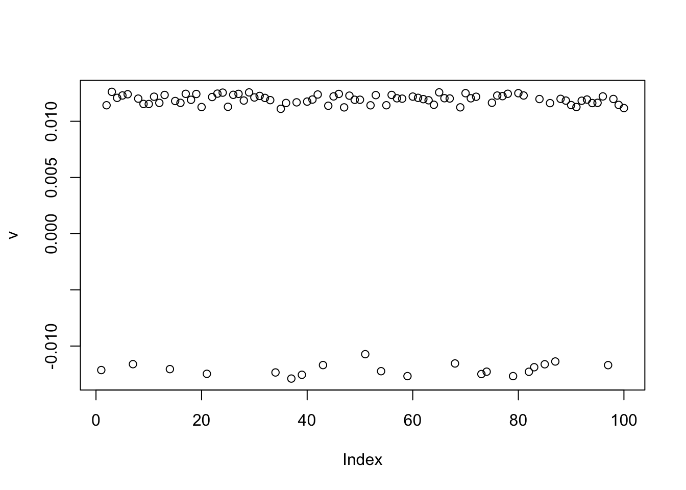

cor(v,L)

           [,1]        [,2]       [,3]
[1,] -0.9990229 -0.01279823 0.07729109

Try instead setting rho=0.5. It converges to a binary source again, but this time close to v in (-1,1).

rho = 0.5
v = v.init
for(i in 1:maxiter){
  v = tanh(P %*% v/(1-rho))
}
t(v) %*% P %*% v/n # print out rho

          [,1]
[1,] 0.9152038

plot(v)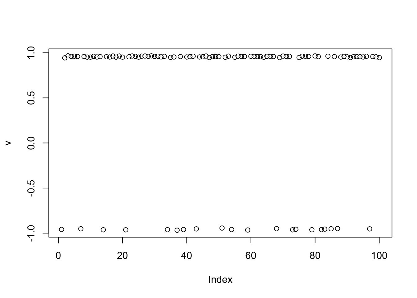

cor(v,L)

           [,1]          [,2]       [,3]
[1,] -0.9999768 -0.0002258368 0.06234581

This time we estimate rho. It converges to a binary source again, but this time close to v in (-1,1).

rho = 0
v = v.init
for(i in 1:maxiter){
  rho = as.numeric(t(v) %*% P %*% v/n) # update rho
  v = tanh(P %*% v/(1-rho))
}
t(v) %*% P %*% v/n # print out rho

          [,1]
[1,] 0.9989868

plot(v)

cor(v,L)

     [,1]          [,2]   [,3]
[1,]   -1 -5.724587e-17 0.0625

Three group simulation (higher noise)

Here I repeat the above, with more noise:

K=3
p = 1000
n = 100
set.seed(1)
L = matrix(-1,nrow=n,ncol=K)
for(i in 1:K){L[sample(1:n,20),i]=1}
FF = matrix(rnorm(p*K), nrow = p, ncol=K)

X = L %*% t(FF) + rnorm(n*p,0,10)

The column space of \(X\) approximately contains three binary vectors (columns of \(L\)). The true value of rho is near 0.8.

U = svd(X)$u[,1:3] 
P = U %*% t(U) 
true_rho = diag(t(L) %*% P %*% L/n)
true_rho

[1] 0.807348 0.790952 0.829372

Now, initializing from a random vector. If we set rho=0 then the iterates converge to something close to 0 (as expected, because tanh is a contraction). This time it does not really find a binary source!

set.seed(1)
v.init.1 = sample(c(-1,1),n,replace=TRUE)
maxiter = 10000

rho = 0
v = v.init.1
for(i in 1:maxiter){
  v = tanh(P %*% v/(1-rho))
}
t(v) %*% P %*% v/n # print out rho

             [,1]
[1,] 8.746538e-05

plot(v)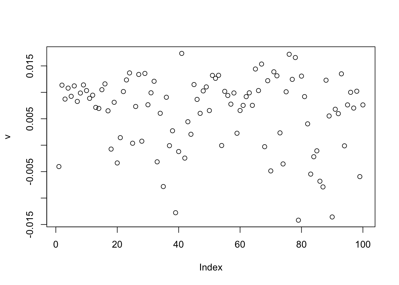

cor(v,L)

          [,1]       [,2]       [,3]
[1,] -0.428421 -0.7348204 0.09921965

Try instead setting rho=0.5. It is getting closer to a binary source.

rho = 0.5
v = v.init.1
for(i in 1:maxiter){
  v = tanh(P %*% v/(1-rho))
}
t(v) %*% P %*% v/n # print out rho

          [,1]
[1,] 0.6826304

plot(v)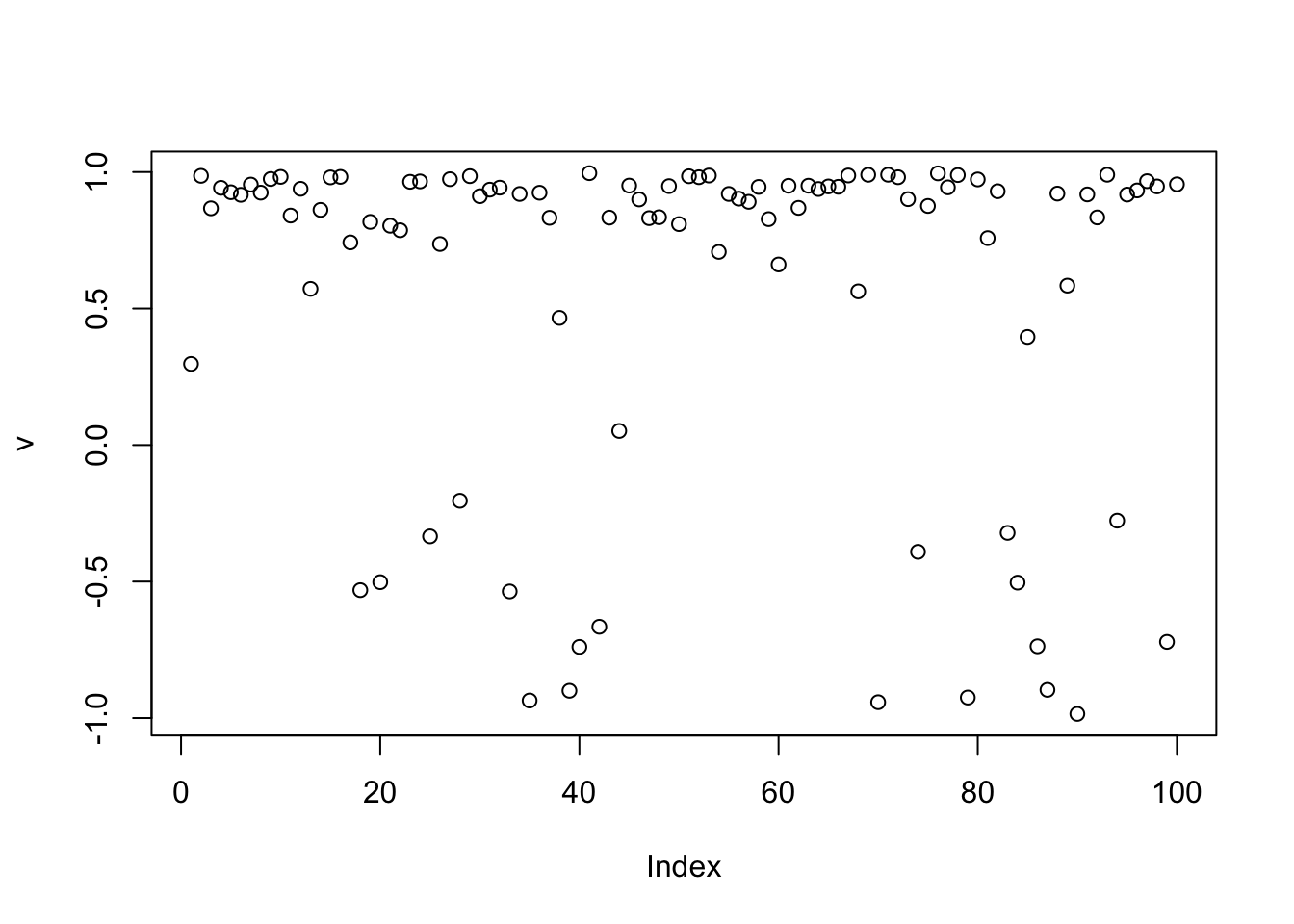

cor(v,L)

           [,1]       [,2]        [,3]
[1,] -0.1350534 -0.8809243 -0.08754405

This time we estimate rho. It converges to something closer to a binary source but does not get it exactly right.

rho = 0
v = v.init.1
for(i in 1:maxiter){
  rho = as.numeric(t(v) %*% P %*% v/n) # update rho
  v = tanh(P %*% v/(1-rho))
}
t(v) %*% P %*% v/n # print out rho

          [,1]
[1,] 0.8272076

plot(v)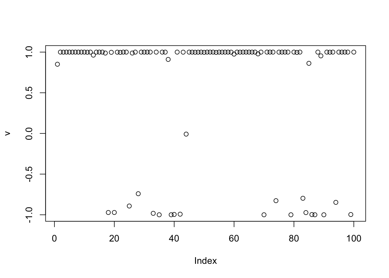

cor(v,L)

            [,1]       [,2]        [,3]
[1,] -0.07294291 -0.8723976 -0.07514556

Try a different random start: it gets closer (and also a larger rho).

set.seed(3)
v.init.3 = sample(c(-1,1),n,replace=TRUE)
rho = 0
v = v.init.3
for(i in 1:maxiter){
  rho = as.numeric(t(v) %*% P %*% v/n) # update rho
  v = tanh(P %*% v/(1-rho))
}
t(v) %*% P %*% v/n # print out rho

          [,1]
[1,] 0.8254599

plot(v)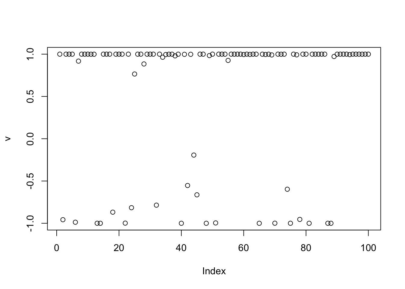

cor(v,L)

           [,1]        [,2]       [,3]
[1,] 0.02204825 -0.07501538 -0.9648287

Try EBICA

set.seed(3)
v.init.3 = sample(c(-1,1),n,replace=TRUE)
rho = 0
v = v.init.3

for(i in 1:maxiter){
  v = tanh(n*P %*% v/as.numeric(sqrt(n * t(v) %*% P %*% v)))
}
t(v) %*% P %*% v/n # print out rho

         [,1]
[1,] 0.487831

plot(v)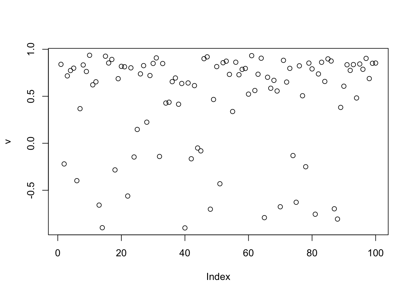

cor(v,L)

           [,1]       [,2]      [,3]
[1,] 0.01389254 -0.1671942 -0.906508

Try centering X

In the above I did not center X. So here I do so. This reduces the “true rho” substantially (below 0.5). The issue is that the original binary vectors are no longer in the subspace spanned by columns of Xcenter - the centering shifts the +-1 vectors so they are no longer +-1.

Xcenter = scale(X,scale=FALSE)
Ucenter = svd(Xcenter)$u[,1:3] 
Pcenter = Ucenter %*% t(Ucenter) 
diag(t(L) %*% Pcenter %*% L/n)

[1] 0.4262193 0.3058118 0.4351670

The method now fails to find them (not suprisingly):

set.seed(3)
v.init.3 = sample(c(-1,1),n,replace=TRUE)
rho = 0
v = v.init.3
for(i in 1:maxiter){
  rho = as.numeric(t(v) %*% Pcenter %*% v/n) # update rho
  v = tanh(Pcenter %*% v/(1-rho))
}
t(v) %*% Pcenter %*% v/n # print out rho

          [,1]
[1,] 0.4034526

plot(v)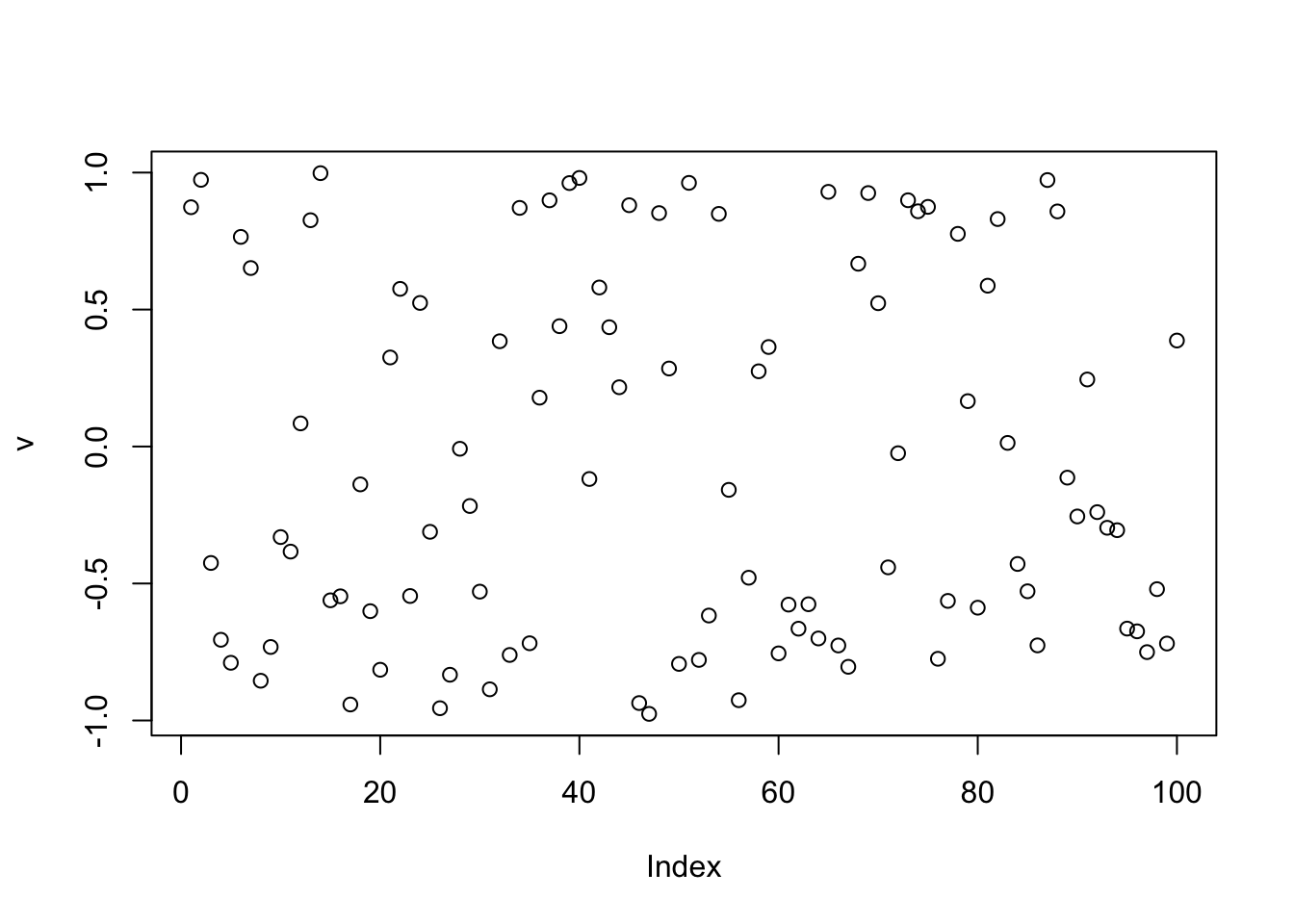

cor(v,L)

          [,1]       [,2]      [,3]
[1,] 0.4690021 0.06030247 0.5967123

If we add an intercept we have a problem: the method finds the trivial solution of all 1s. (When I ran this about five times with different seeds it did eventually find one of the sources. But the trivial solution has the largest rho, so it tends to win.)

Ucenter = cbind(rep(1/sqrt(n),n),Ucenter) # add an intercept
Pcenter = Ucenter %*% t(Ucenter) 
diag(t(L) %*% Pcenter %*% L/n) #rho is back to 0.8 or so

[1] 0.7862193 0.6658118 0.7951670

set.seed(3)
v.init.3 = sample(c(-1,1),n,replace=TRUE)
rho = 0
v = v.init.3
v = sample(c(-1,1),n,replace=TRUE)
for(i in 1:maxiter){
  rho = as.numeric(t(v) %*% Pcenter %*% v/n) # update rho
  v = tanh(Pcenter %*% v/(1-rho))
}
t(v) %*% Pcenter %*% v/n # print out rho

     [,1]
[1,]    1

plot(v)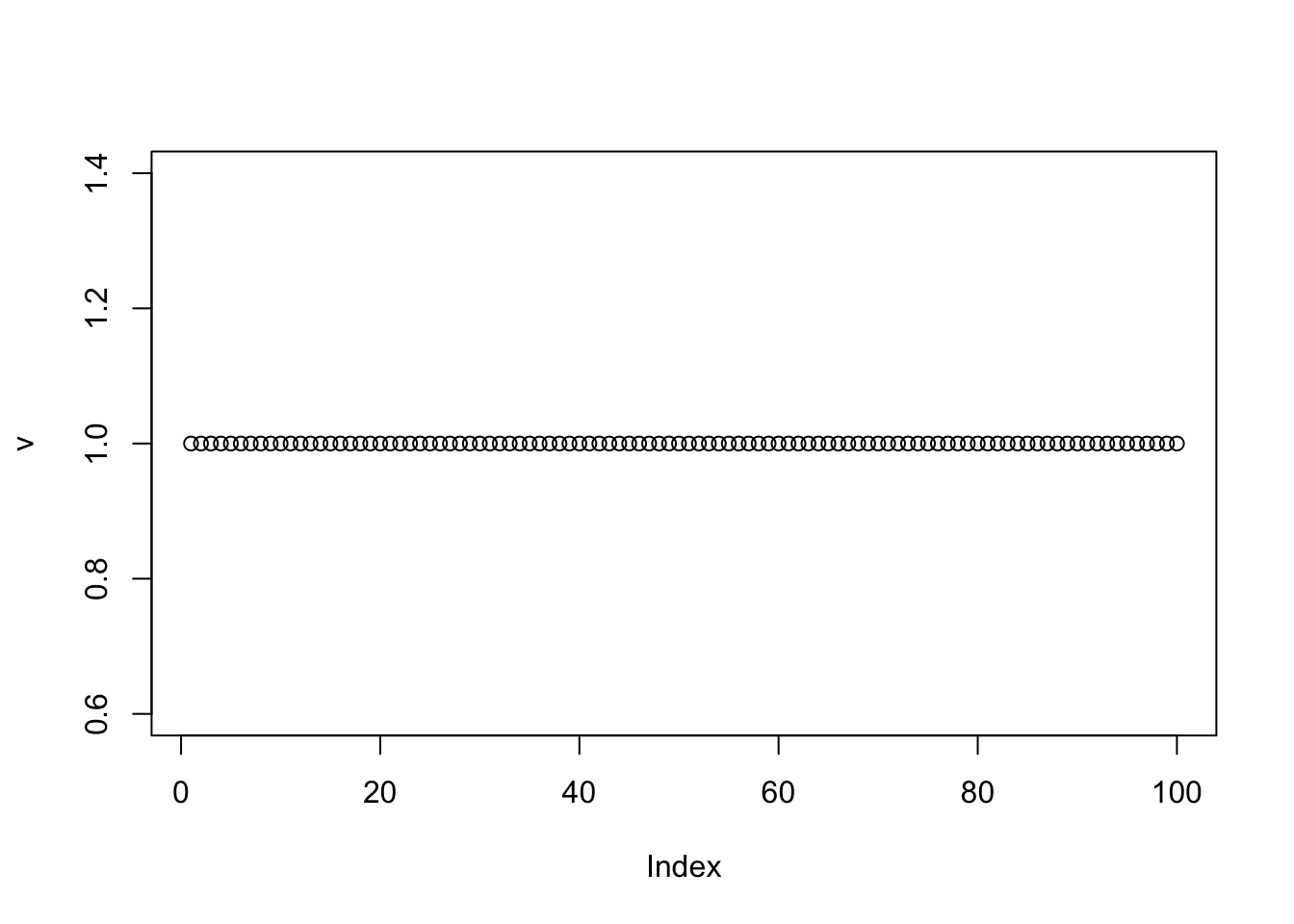

cor(v,L)

Warning in cor(v, L): the standard deviation is zero

     [,1] [,2] [,3]
[1,]   NA   NA   NA

sessionInfo()

R version 4.4.2 (2024-10-31)
Platform: aarch64-apple-darwin20
Running under: macOS Sequoia 15.6.1

Matrix products: default
BLAS:   /System/Library/Frameworks/Accelerate.framework/Versions/A/Frameworks/vecLib.framework/Versions/A/libBLAS.dylib 
LAPACK: /Library/Frameworks/R.framework/Versions/4.4-arm64/Resources/lib/libRlapack.dylib;  LAPACK version 3.12.0

locale:
[1] en_US.UTF-8/en_US.UTF-8/en_US.UTF-8/C/en_US.UTF-8/en_US.UTF-8

time zone: America/Chicago
tzcode source: internal

attached base packages:
[1] stats     graphics  grDevices utils     datasets  methods   base     

loaded via a namespace (and not attached):
 [1] vctrs_0.7.2       cli_3.6.5         knitr_1.51        rlang_1.1.7      
 [5] xfun_0.56         stringi_1.8.7     otel_0.2.0        promises_1.5.0   
 [9] jsonlite_2.0.0    workflowr_1.7.2   glue_1.8.0        rprojroot_2.1.1  
[13] git2r_0.36.2      htmltools_0.5.9   httpuv_1.6.16     sass_0.4.10      
[17] rmarkdown_2.30    jquerylib_0.1.4   evaluate_1.0.5    tibble_3.3.1     
[21] fastmap_1.2.0     yaml_2.3.12       lifecycle_1.0.5   whisker_0.4.1    
[25] stringr_1.6.0     compiler_4.4.2    fs_1.6.6          Rcpp_1.1.1       
[29] pkgconfig_2.0.3   rstudioapi_0.18.0 later_1.4.6       digest_0.6.39    
[33] R6_2.6.1          pillar_1.11.1     magrittr_2.0.4    bslib_0.10.0     
[37] tools_4.4.2       cachem_1.1.0

EB_subspace

Matthew Stephens

2026-06-19

Introduction

Three group simulation (low noise)

Three group simulation (higher noise)

Try centering X