Gaussian process
Matthew Stephens
5/21/2018
Last updated: 2018-05-21
workflowr checks: (Click a bullet for more information)-
✔ R Markdown file: up-to-date
Great! Since the R Markdown file has been committed to the Git repository, you know the exact version of the code that produced these results.
-
✔ Environment: empty
Great job! The global environment was empty. Objects defined in the global environment can affect the analysis in your R Markdown file in unknown ways. For reproduciblity it’s best to always run the code in an empty environment.
-
✔ Seed:
set.seed(20180411)The command
set.seed(20180411)was run prior to running the code in the R Markdown file. Setting a seed ensures that any results that rely on randomness, e.g. subsampling or permutations, are reproducible. -
✔ Session information: recorded
Great job! Recording the operating system, R version, and package versions is critical for reproducibility.
-
Great! You are using Git for version control. Tracking code development and connecting the code version to the results is critical for reproducibility. The version displayed above was the version of the Git repository at the time these results were generated.✔ Repository version: f4a663d
Note that you need to be careful to ensure that all relevant files for the analysis have been committed to Git prior to generating the results (you can usewflow_publishorwflow_git_commit). workflowr only checks the R Markdown file, but you know if there are other scripts or data files that it depends on. Below is the status of the Git repository when the results were generated:
Note that any generated files, e.g. HTML, png, CSS, etc., are not included in this status report because it is ok for generated content to have uncommitted changes.Ignored files: Ignored: .DS_Store Ignored: .Rhistory Ignored: .Rproj.user/ Ignored: .sos/ Ignored: exams/ Ignored: temp/ Untracked files: Untracked: analysis/hmm.Rmd Untracked: analysis/neanderthal.Rmd Untracked: analysis/pca_cell_cycle.Rmd Untracked: analysis/ridge_mle.Rmd Untracked: data/reduced.chr12.90-100.data.txt Untracked: data/reduced.chr12.90-100.snp.txt Untracked: docs/figure/hmm.Rmd/ Untracked: docs/figure/pca_cell_cycle.Rmd/ Untracked: homework/fdr.aux Untracked: homework/fdr.log Untracked: tempETA_1_parBayesC.dat Untracked: temp_ETA_1_parBayesC.dat Untracked: temp_mu.dat Untracked: temp_varE.dat Untracked: tempmu.dat Untracked: tempvarE.dat Unstaged changes: Modified: analysis/cell_cycle.Rmd Modified: analysis/density_est_cell_cycle.Rmd Modified: analysis/eb_vs_soft.Rmd Modified: analysis/eight_schools.Rmd Modified: analysis/glmnet_intro.Rmd
Expand here to see past versions:
Simulate Gaussian Process
Here we simulate a GP with squared exponential kernel:
set.seed(1)
x = seq(0,1,length=100)
d = abs(outer(x,x,"-")) # compute distance matrix, d_{ij} = |x_i - x_j|
l = 1 # length scale
Sigma_SE = exp(-d^2/(2*l^2)) # squared exponential kernel
y = mvtnorm::rmvnorm(1,sigma=Sigma_SE)
plot(x,y)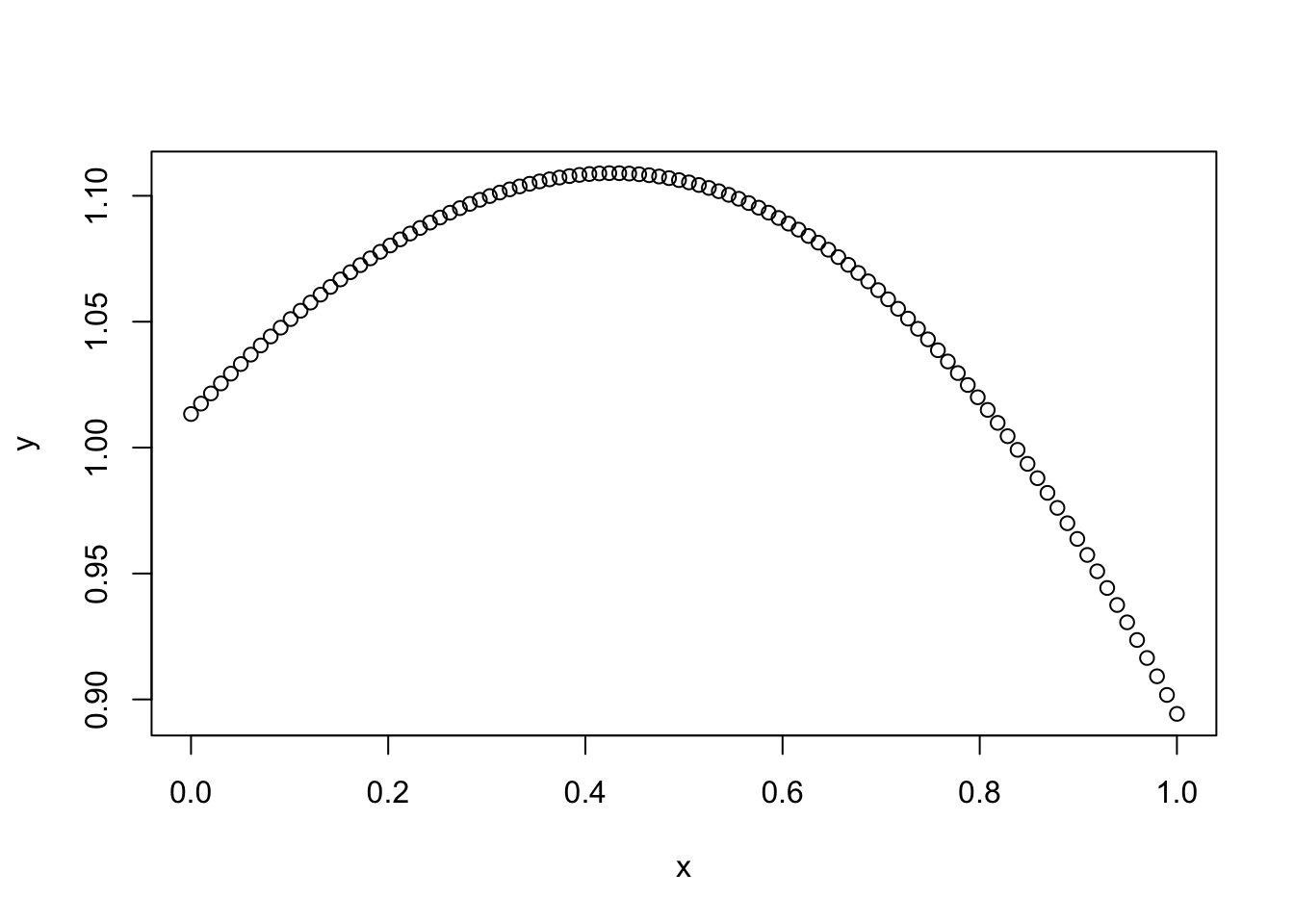
Expand here to see past versions of unnamed-chunk-1-1.png:
| Version | Author | Date |
|---|---|---|
| 4d2b236 | stephens999 | 2018-05-21 |
Try making the covariance decay faster with distance:
l = 0.1
Sigma_SE = exp(-d^2/(2*l^2)) # squared exponential kernel
y = mvtnorm::rmvnorm(1,sigma=Sigma_SE)
plot(x,y)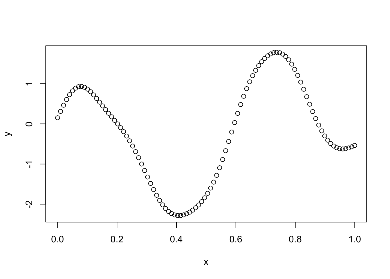
Expand here to see past versions of unnamed-chunk-2-1.png:
| Version | Author | Date |
|---|---|---|
| 4d2b236 | stephens999 | 2018-05-21 |
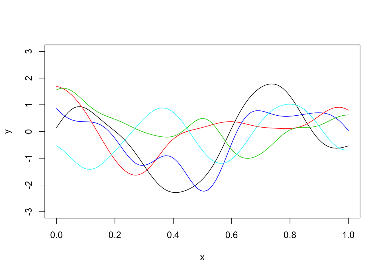
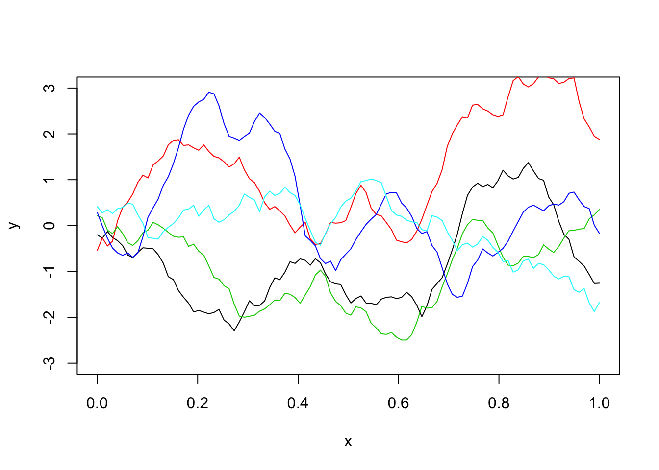
Here is a plot of five different simulations:
plot(x,y,type="l",ylim=c(-3,3))
for(i in 1:4){
  y = mvtnorm::rmvnorm(1,sigma=Sigma_SE)
  lines(x,y,col=i+1)
}
Expand here to see past versions of unnamed-chunk-3-1.png:
| Version | Author | Date |
|---|---|---|
| 4d2b236 | stephens999 | 2018-05-21 |
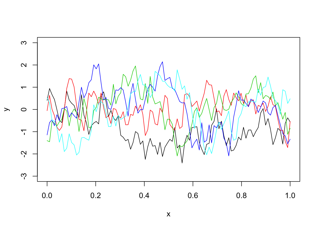
The OU covariance function:
Here we use the covariance function for what is known as the “Ornstein–Uhlenbeck process”, which you can think of as a modified Brownian motion, where the modification tends to pull the process back towards 0. (Unmodified BM tends to wander progressively further from 0.)
Notice it produces much “rougher” functions (actually not differentiable)!
Sigma_OU = exp(-d/l) # OU kernel
y = mvtnorm::rmvnorm(1,sigma=Sigma_OU)
plot(x,y,type="l",ylim=c(-3,3))
for(i in 1:4){
  y = mvtnorm::rmvnorm(1,sigma=Sigma_OU)
  lines(x,y,col=i+1)
}
Expand here to see past versions of unnamed-chunk-4-1.png:
| Version | Author | Date |
|---|---|---|
| 4d2b236 | stephens999 | 2018-05-21 |
Matern covariance function
library("geoR")--------------------------------------------------------------
Analysis of Geostatistical Data
For an Introduction to geoR go to http://www.leg.ufpr.br/geoR
geoR version 1.7-5.2 (built on 2016-05-02) is now loaded
--------------------------------------------------------------Sigma_M = matern(d,phi=l,kappa=1)
y = mvtnorm::rmvnorm(1,sigma=Sigma_M)
plot(x,y,type="l",ylim=c(-3,3))
for(i in 1:4){
y = mvtnorm::rmvnorm(1,sigma=Sigma_M)
lines(x,y,col=i+1)
}
Expand here to see past versions of unnamed-chunk-5-1.png:
| Version | Author | Date |
|---|---|---|
| 4d2b236 | stephens999 | 2018-05-21 |
Eigen-decompositions
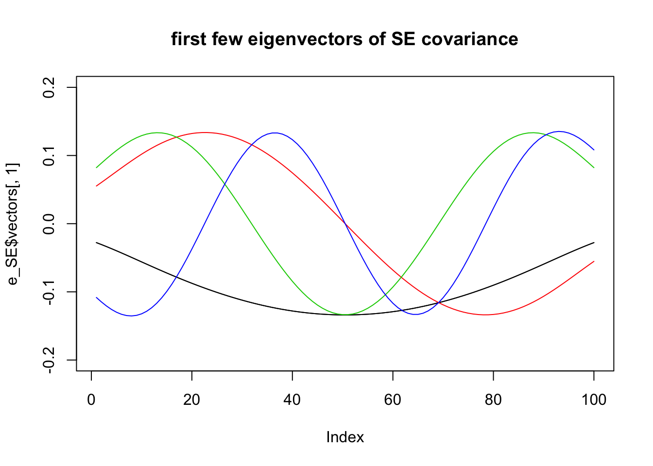
Recall that every covariance matrix \(\Sigma\) has an eigen-decomposition of the form: \[\Sigma = \sum_i \lambda_i v_i v_i' \] where the \(v_i\) are the eigenvectors of \(\Sigma\) and \(\lambda_i\) are the corresponding eigenvalues.
Here we plot the first few eigenvectors of the different covariance matrices.
For the squared exponential:
e_SE = eigen(Sigma_SE)
plot(e_SE$vectors[,1],type="l",ylim=c(-.2,.2),main="first few eigenvectors of SE covariance")
for(i in 1:4){
  lines(e_SE$vectors[,i],col=i)
}
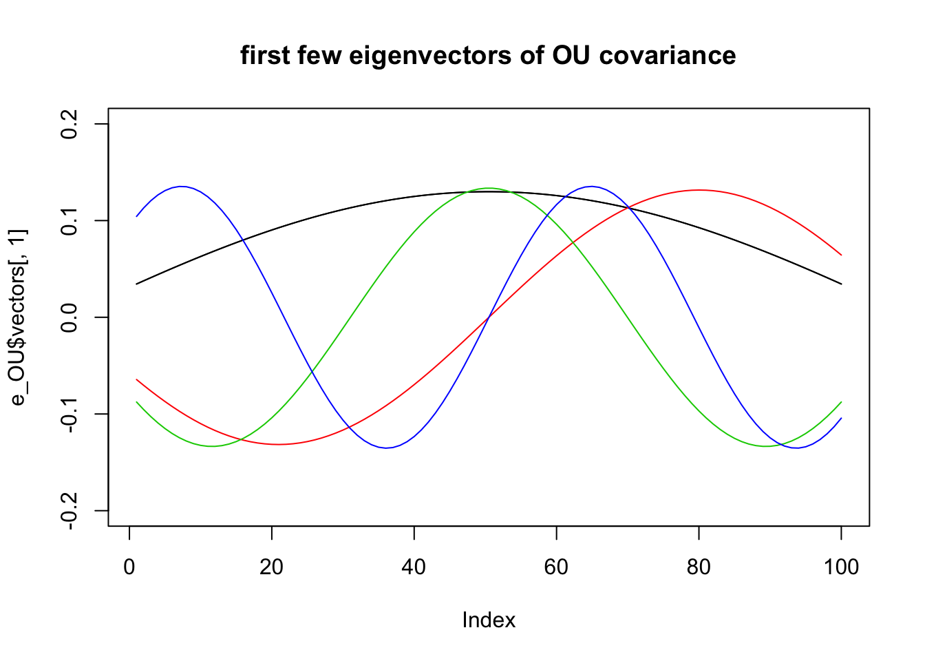
For the OU:
e_OU = eigen(Sigma_OU)
plot(e_OU$vectors[,1],type="l",ylim=c(-.2,.2),main="first few eigenvectors of OU covariance")
for(i in 1:4){
  lines(e_OU$vectors[,i],col=i)
}
And here are the 30th eigenvectors in each case
plot(e_SE$vectors[,30],type="l",ylim=c(-.2,.2))
lines(e_OU$vectors[,30],col=2,ylim=c(-.2,.2))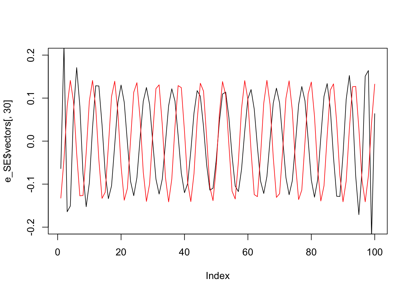
So the eigenvectors are kind of “similar” in each case. (There is a reason for this: the matrices are close to “circulant” and all \(n \times n\) circulant matries have the same eigenvectors, which are the columns of the discrete Fourier transform matrix).
Notice how the eigenvalues are very different.
plot(e_SE$values,type="l",main="eigenvalues of SE (black) and OU (red)")
lines(e_OU$values,col=2)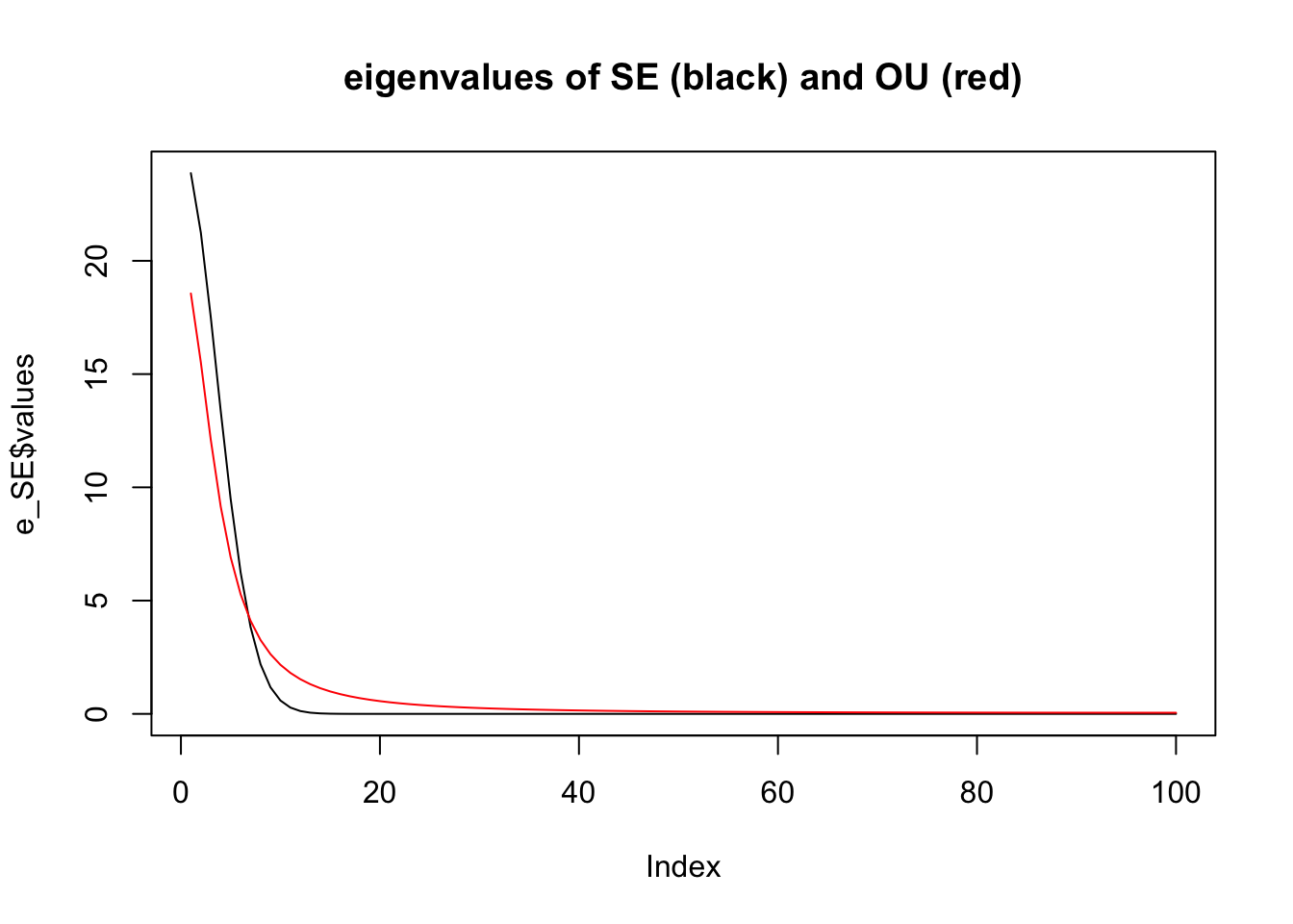
Especially if we look closely at the small eigenvalues:
plot(e_SE$values,type="l",ylim=c(0,0.4),main="eigenvalues of SE (black) and OU (red)")
lines(e_OU$values,col=2)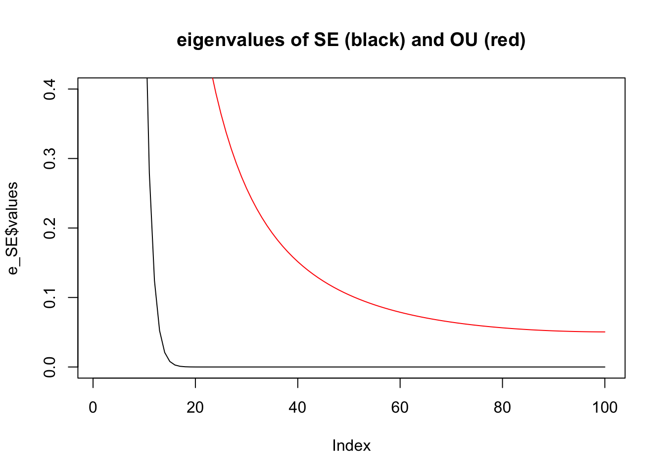
Note: the higher eigenvalues of \(\Sigma_{SE}\) are very close to machine precision, so the corresponding eigenvectors should probably not be trusted!
Session information
sessionInfo()R version 3.3.2 (2016-10-31)
Platform: x86_64-apple-darwin13.4.0 (64-bit)
Running under: OS X El Capitan 10.11.6
locale:
[1] en_US.UTF-8/en_US.UTF-8/en_US.UTF-8/C/en_US.UTF-8/en_US.UTF-8
attached base packages:
[1] stats graphics grDevices utils datasets methods base
other attached packages:
[1] geoR_1.7-5.2
loaded via a namespace (and not attached):
[1] Rcpp_0.12.16 knitr_1.20
[3] whisker_0.3-2 magrittr_1.5
[5] workflowr_1.0.1 MASS_7.3-49
[7] lattice_0.20-35 stringr_1.3.0
[9] tcltk_3.3.2 tools_3.3.2
[11] RandomFields_3.1.50 grid_3.3.2
[13] R.oo_1.22.0 git2r_0.21.0
[15] RandomFieldsUtils_0.3.25 htmltools_0.3.6
[17] yaml_2.1.18 rprojroot_1.3-2
[19] digest_0.6.15 splancs_2.01-40
[21] R.utils_2.6.0 evaluate_0.10.1
[23] rmarkdown_1.9 sp_1.2-7
[25] stringi_1.1.7 backports_1.1.2
[27] R.methodsS3_1.7.1 mvtnorm_1.0-7 This reproducible R Markdown analysis was created with workflowr 1.0.1