histogram for cell cycle
Matthew Stephens
April 11, 2018
Last updated: 2018-05-21
workflowr checks: (Click a bullet for more information)-
✔ R Markdown file: up-to-date
Great! Since the R Markdown file has been committed to the Git repository, you know the exact version of the code that produced these results.
-
✔ Environment: empty
Great job! The global environment was empty. Objects defined in the global environment can affect the analysis in your R Markdown file in unknown ways. For reproduciblity it’s best to always run the code in an empty environment.
-
✔ Seed:
set.seed(20180411)The command
set.seed(20180411)was run prior to running the code in the R Markdown file. Setting a seed ensures that any results that rely on randomness, e.g. subsampling or permutations, are reproducible. -
✔ Session information: recorded
Great job! Recording the operating system, R version, and package versions is critical for reproducibility.
-
Great! You are using Git for version control. Tracking code development and connecting the code version to the results is critical for reproducibility. The version displayed above was the version of the Git repository at the time these results were generated.✔ Repository version: 34e295c
Note that you need to be careful to ensure that all relevant files for the analysis have been committed to Git prior to generating the results (you can usewflow_publishorwflow_git_commit). workflowr only checks the R Markdown file, but you know if there are other scripts or data files that it depends on. Below is the status of the Git repository when the results were generated:
Note that any generated files, e.g. HTML, png, CSS, etc., are not included in this status report because it is ok for generated content to have uncommitted changes.Ignored files: Ignored: .DS_Store Ignored: .Rhistory Ignored: .Rproj.user/ Ignored: .sos/ Ignored: exams/ Ignored: temp/ Untracked files: Untracked: analysis/hmm.Rmd Untracked: analysis/neanderthal.Rmd Untracked: analysis/pca_cell_cycle.Rmd Untracked: analysis/ridge_mle.Rmd Untracked: data/reduced.chr12.90-100.data.txt Untracked: data/reduced.chr12.90-100.snp.txt Untracked: docs/figure/hmm.Rmd/ Untracked: docs/figure/pca_cell_cycle.Rmd/ Untracked: homework/fdr.aux Untracked: homework/fdr.log Untracked: tempETA_1_parBayesC.dat Untracked: temp_ETA_1_parBayesC.dat Untracked: temp_mu.dat Untracked: temp_varE.dat Untracked: tempmu.dat Untracked: tempvarE.dat Unstaged changes: Modified: analysis/cell_cycle.Rmd Modified: analysis/eb_vs_soft.Rmd Modified: analysis/svd_zip.Rmd
Expand here to see past versions:
Introduction
We will try estimating the density of the cell cycle values. See (cell_cycle.Rmd) for more on those data.
Histograms
First we try histograms. The histograms here are un-normalized, so not actually densities. We could normalize them easily enough, but I think it is helpful for you to see the counts get smaller.
Let’s start with the default:
d = readRDS("../data/cyclegenes.rds")
hist(d[,1],xlab="theta (cell cycle position)", main="Histogram of theta")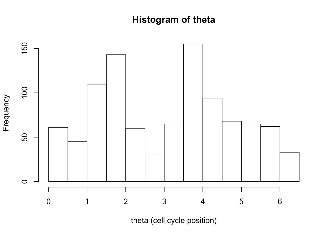
And now try decreasing bin sizes to see the bias/variance trade-off in action.
hist(d[,1],breaks = seq(0,2*pi,length=5),xlab="theta (cell cycle position)", main="Histogram of theta")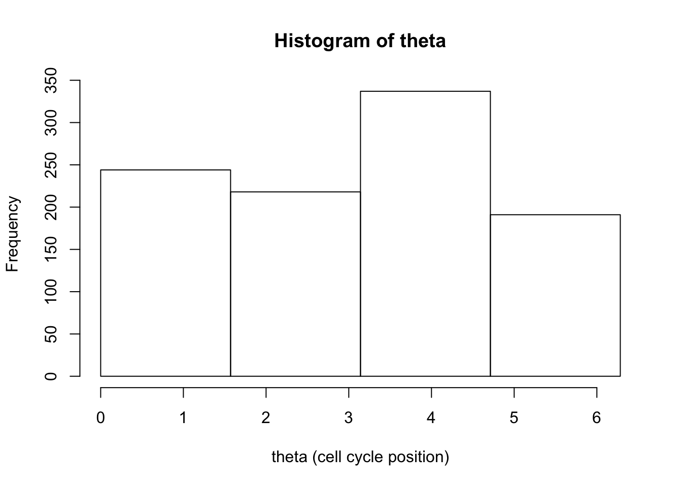
hist(d[,1],breaks = seq(0,2*pi,length=20),xlab="theta (cell cycle position)", main="Histogram of theta")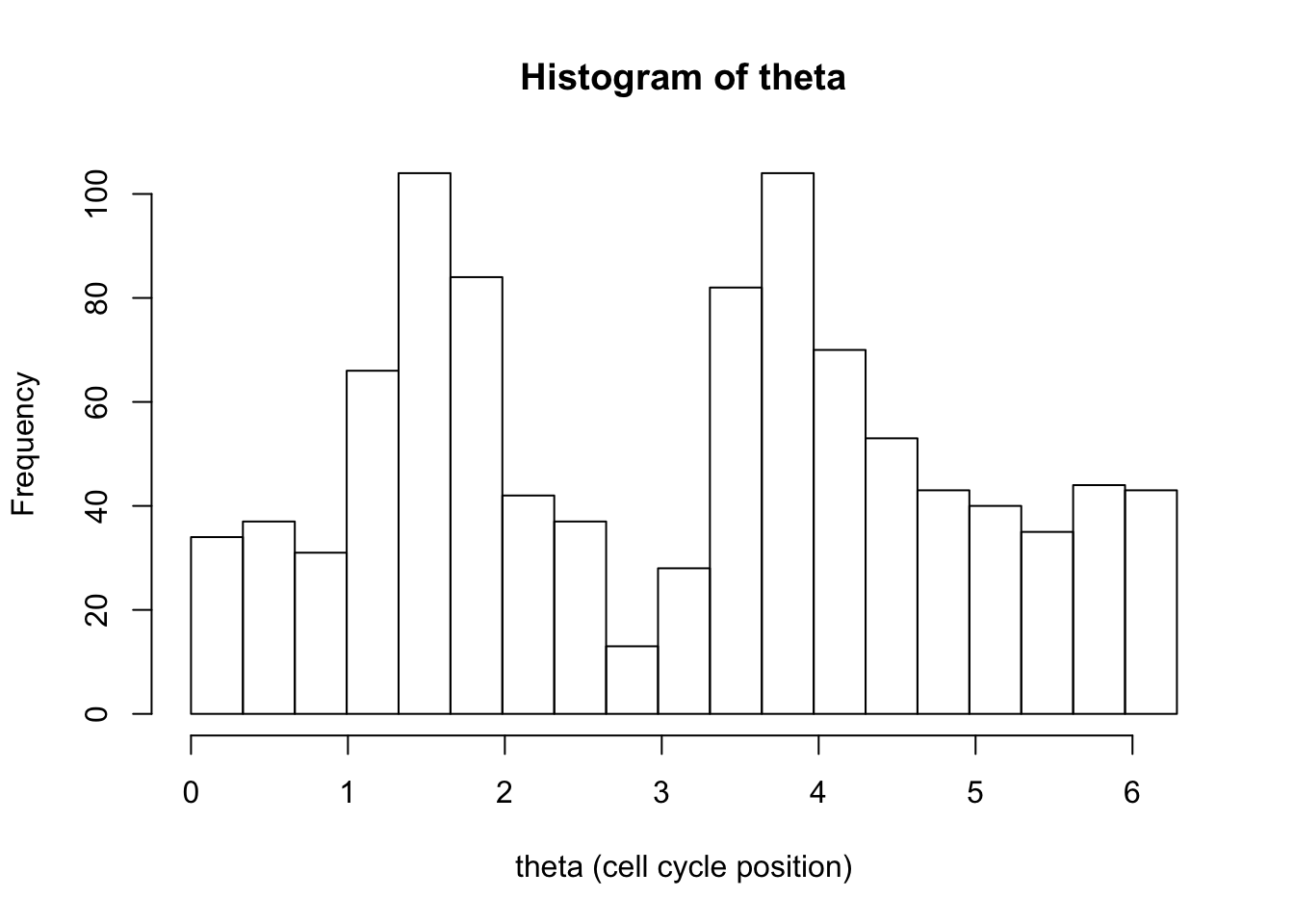
hist(d[,1],breaks = seq(0,2*pi,length=100),xlab="theta (cell cycle position)", main="Histogram of theta")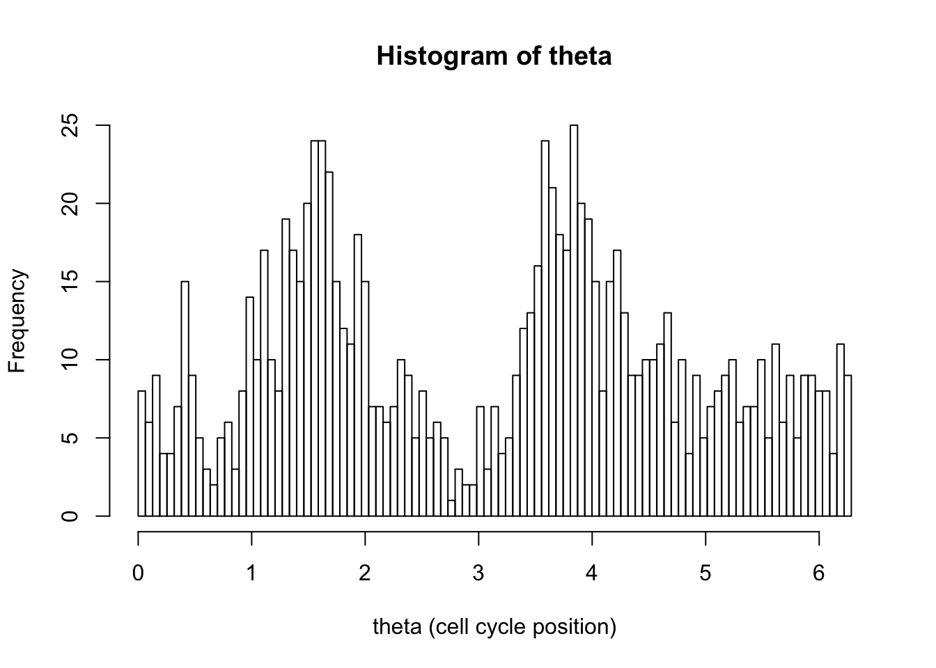
hist(d[,1],breaks = seq(0,2*pi,length=400),xlab="theta (cell cycle position)", main="Histogram of theta")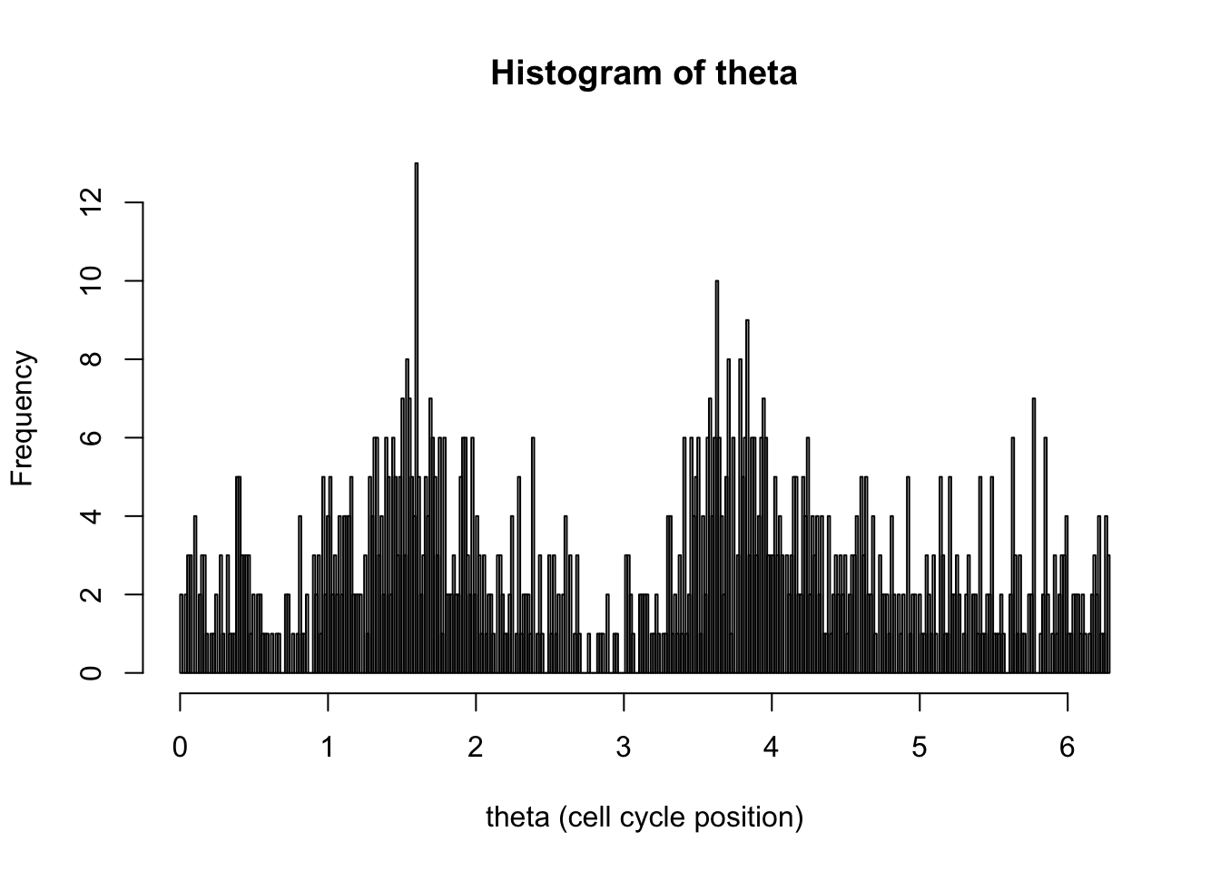
hist(d[,1],breaks = seq(0,2*pi,length=1000),xlab="theta (cell cycle position)", main="Histogram of theta")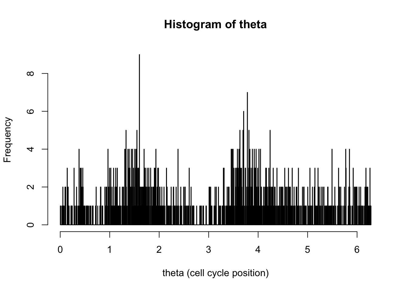
Density estimation
Let’s try the default density estimation in the R function “density”.
hist(d[,1],breaks = seq(0,2*pi,length=100),xlab="theta (cell cycle position)", main="Histogram of theta",probability=TRUE)
d.dens = density(d[,1])
lines(d.dens$x,d.dens$y,col=2,lwd=2)
The analogue of bin size is “bandwidth”, set using bw. Here we try four very different bandwidths.
hist(d[,1],breaks = seq(0,2*pi,length=100),xlab="theta (cell cycle position)", main="Histogram of theta",probability=TRUE)
d1.dens = density(d[,1],bw=0.01)
d2.dens = density(d[,1],bw=0.1)
d3.dens = density(d[,1],bw=1)
d4.dens = density(d[,1],bw=10)

lines(d1.dens$x,d1.dens$y,col=2,lwd=2)
lines(d2.dens$x,d2.dens$y,col=3,lwd=2)
lines(d3.dens$x,d3.dens$y,col=4,lwd=2)
lines(d4.dens$x,d4.dens$y,col=5,lwd=2)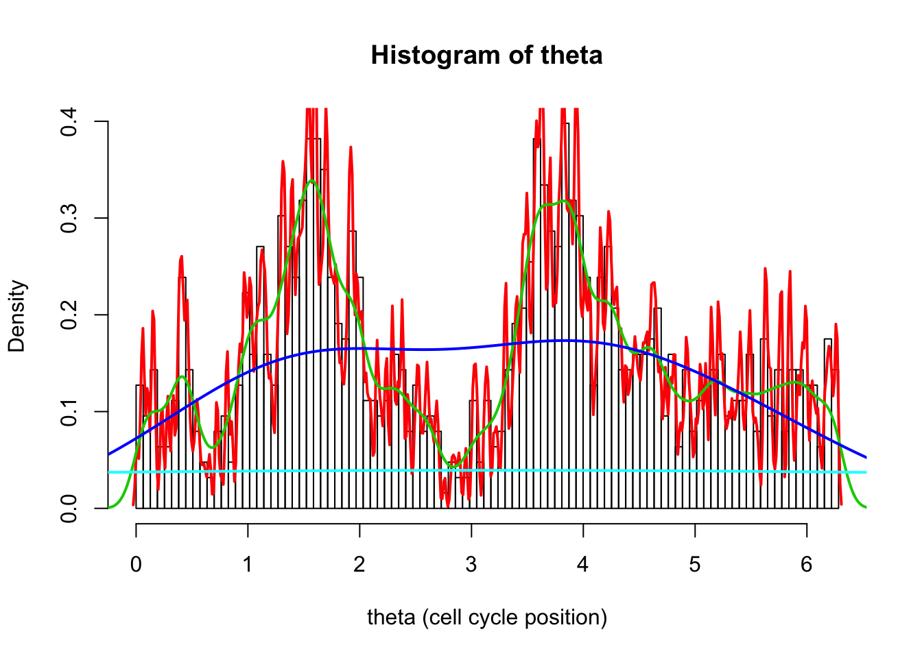
A common issue with density
Go back to the origin plot.
hist(d[,1],breaks = seq(0,2*pi,length=100),xlab="theta (cell cycle position)", main="Histogram of theta",probability=TRUE)
d.dens = density(d[,1])
lines(d.dens$x,d.dens$y,col=2,lwd=2)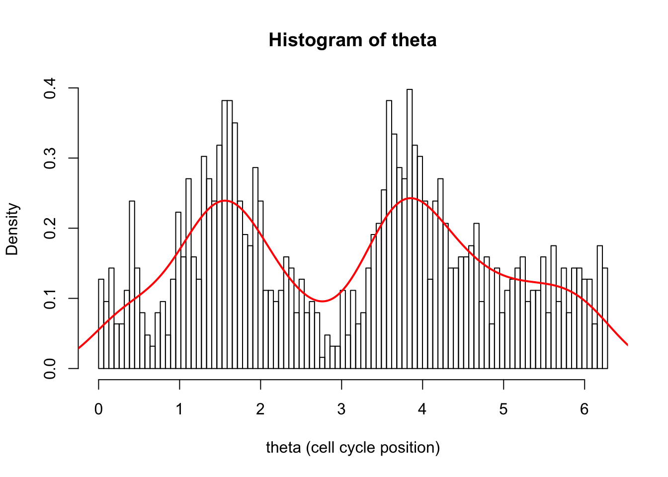
Notice how the density seems too low at both ends of the plot. This is a common problem with density when applied to a finite domain like this. It is because it is estimating the density at 0 and notices there are no observations just to the left of 0, and this biases the estimate of density down.
We can see the problem better if we plot a wider area:
hist(d[,1],breaks = seq(-pi,3*pi,length=100),xlab="theta (cell cycle position)", main="Histogram of theta",probability=TRUE)
d.dens = density(d[,1])
lines(d.dens$x,d.dens$y,col=2,lwd=2)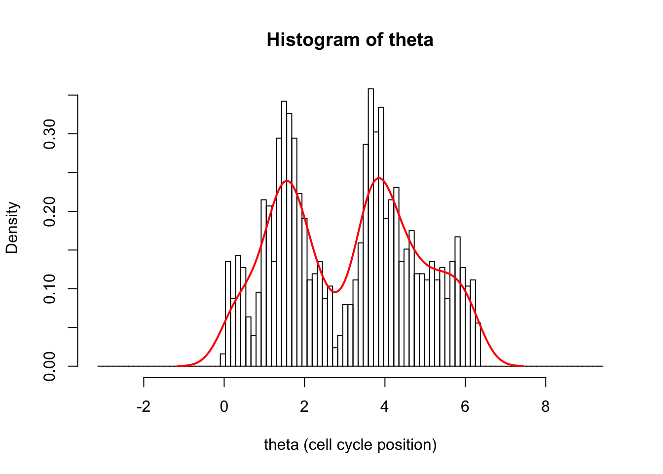
To deal with this a simple trick is to reflect the data at both ends.
x = d[,1]
x = c(-x,x,2*pi + 2*pi-x)
hist(x,prob=TRUE)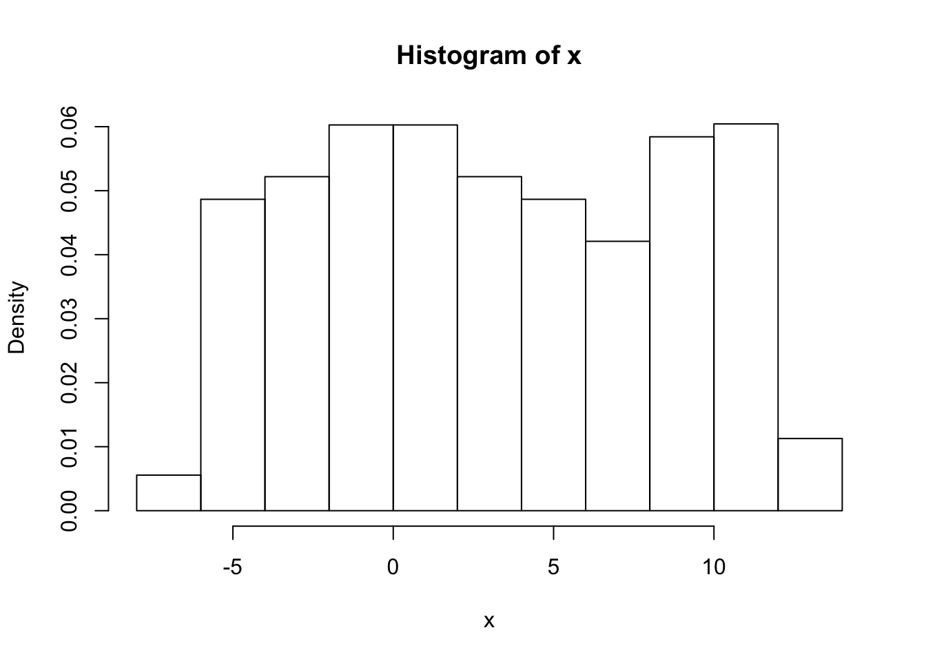
er… yuk! the default histogram was not very nice - have to do it by hand!
hist(x,breaks = seq(-2*pi, 4*pi,length=100),probability=TRUE)
abline(v=0,col=2)
abline(v=2*pi,col=2)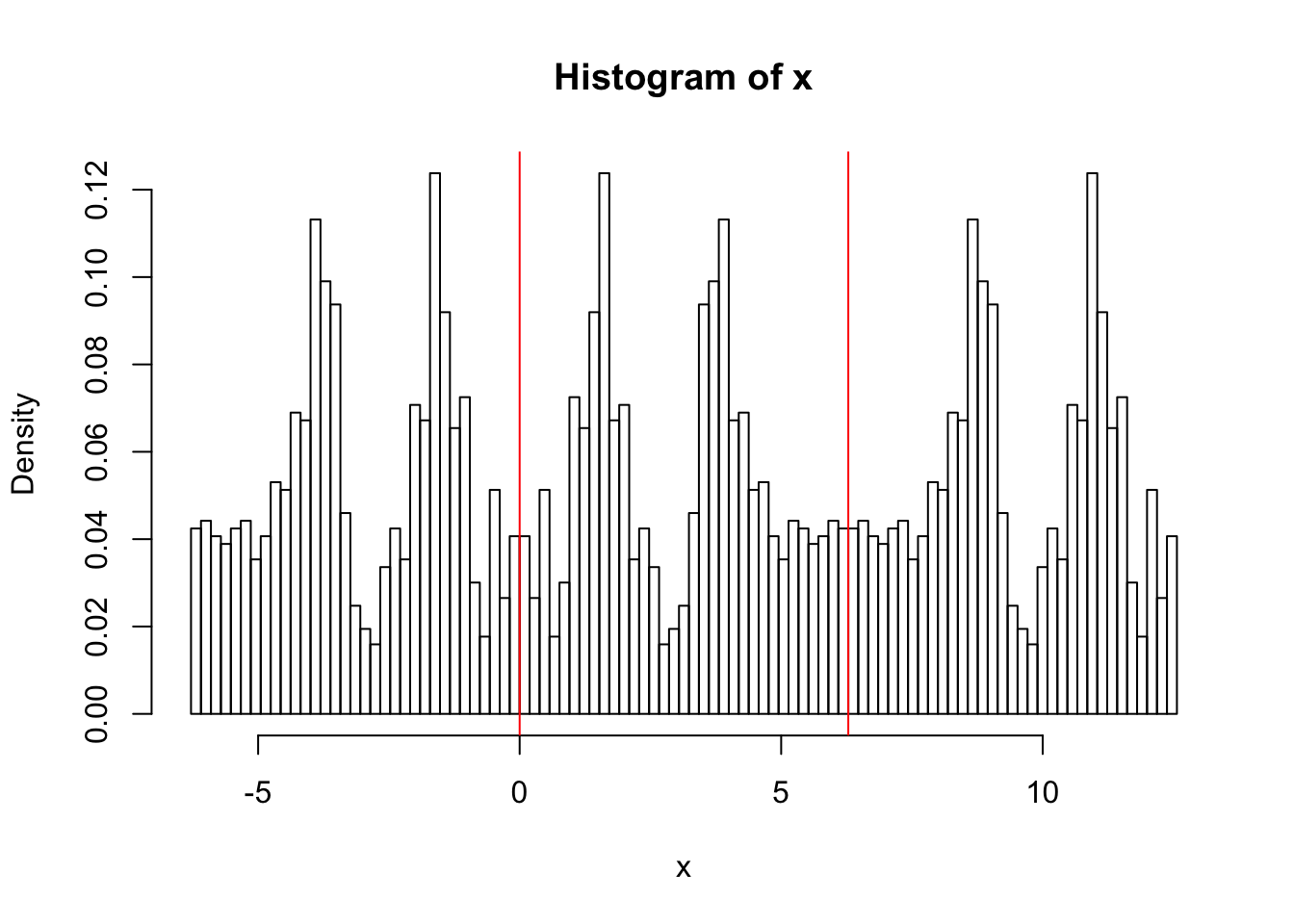
So now we can estimate the density
x.dens = density(x)
hist(x,breaks = seq(-2*pi, 4*pi,length=100),probability=TRUE)
abline(v=0,col=2)
abline(v=2*pi,col=2)
lines(x.dens$x,x.dens$y,col=2)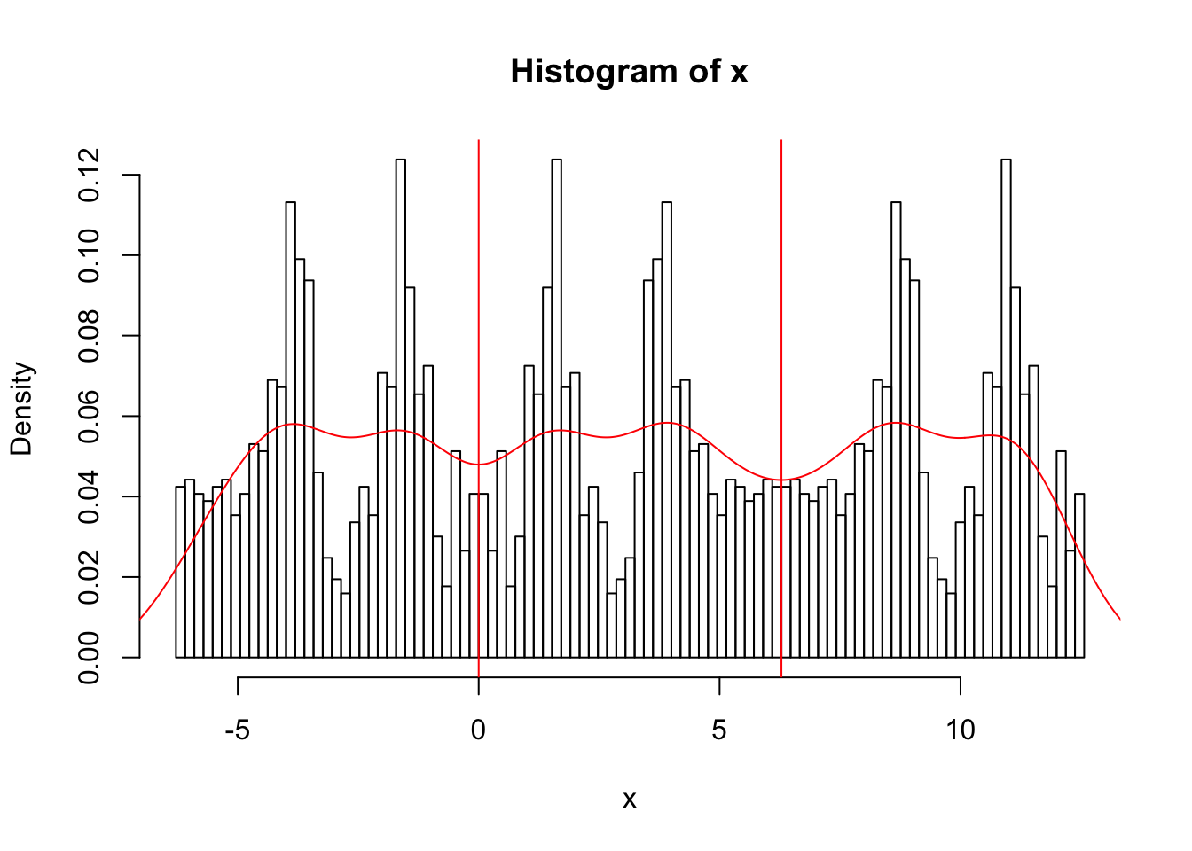
Also yuk!! I had to experiment with the parameter bw to get a nicer plot….
x.dens = density(x,bw=0.2)
hist(x,breaks = seq(-2*pi, 4*pi,length=100),probability=TRUE)
abline(v=0,col=2)
abline(v=2*pi,col=2)
lines(x.dens$x,x.dens$y,col=3)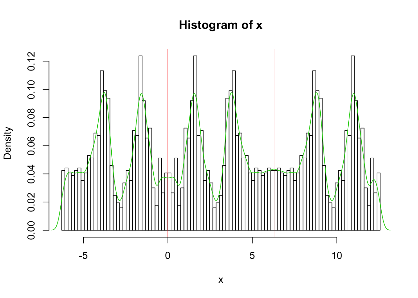
I now could get a nice density estimate in the range 0 to 2pi by just truncating and renormalizing to have area 1.
Session information
sessionInfo()R version 3.3.2 (2016-10-31)
Platform: x86_64-apple-darwin13.4.0 (64-bit)
Running under: OS X El Capitan 10.11.6
locale:
[1] en_US.UTF-8/en_US.UTF-8/en_US.UTF-8/C/en_US.UTF-8/en_US.UTF-8
attached base packages:
[1] stats graphics grDevices utils datasets methods base
loaded via a namespace (and not attached):
[1] workflowr_1.0.1 Rcpp_0.12.16 digest_0.6.15
[4] rprojroot_1.3-2 R.methodsS3_1.7.1 backports_1.1.2
[7] git2r_0.21.0 magrittr_1.5 evaluate_0.10.1
[10] stringi_1.1.7 whisker_0.3-2 R.oo_1.22.0
[13] R.utils_2.6.0 rmarkdown_1.9 tools_3.3.2
[16] stringr_1.3.0 yaml_2.1.18 htmltools_0.3.6
[19] knitr_1.20 This reproducible R Markdown analysis was created with workflowr 1.0.1