shrinkage
Matthew Stephens
April 9, 2018
Last updated: 2018-05-21
workflowr checks: (Click a bullet for more information)-
✔ R Markdown file: up-to-date
Great! Since the R Markdown file has been committed to the Git repository, you know the exact version of the code that produced these results.
-
✔ Environment: empty
Great job! The global environment was empty. Objects defined in the global environment can affect the analysis in your R Markdown file in unknown ways. For reproduciblity it’s best to always run the code in an empty environment.
-
✔ Seed:
set.seed(20180411)The command
set.seed(20180411)was run prior to running the code in the R Markdown file. Setting a seed ensures that any results that rely on randomness, e.g. subsampling or permutations, are reproducible. -
✔ Session information: recorded
Great job! Recording the operating system, R version, and package versions is critical for reproducibility.
-
Great! You are using Git for version control. Tracking code development and connecting the code version to the results is critical for reproducibility. The version displayed above was the version of the Git repository at the time these results were generated.✔ Repository version: 5b61f90
Note that you need to be careful to ensure that all relevant files for the analysis have been committed to Git prior to generating the results (you can usewflow_publishorwflow_git_commit). workflowr only checks the R Markdown file, but you know if there are other scripts or data files that it depends on. Below is the status of the Git repository when the results were generated:
Note that any generated files, e.g. HTML, png, CSS, etc., are not included in this status report because it is ok for generated content to have uncommitted changes.Ignored files: Ignored: .DS_Store Ignored: .Rhistory Ignored: .Rproj.user/ Ignored: .sos/ Ignored: exams/ Ignored: temp/ Untracked files: Untracked: analysis/neanderthal.Rmd Untracked: analysis/pca_cell_cycle.Rmd Untracked: analysis/ridge_mle.Rmd Untracked: data/reduced.chr12.90-100.data.txt Untracked: data/reduced.chr12.90-100.snp.txt Untracked: docs/figure/pca_cell_cycle.Rmd/ Untracked: homework/fdr.aux Untracked: homework/fdr.log Untracked: tempETA_1_parBayesC.dat Untracked: temp_ETA_1_parBayesC.dat Untracked: temp_mu.dat Untracked: temp_varE.dat Untracked: tempmu.dat Untracked: tempvarE.dat
Expand here to see past versions:
Simulate some data
Here we simulate a pretty sparse situation: 90% sparsity.
set.seed(1)
theta = c(rep(0,900),rnorm(100,0,4))
x = theta + rnorm(1000)
hist(theta,breaks = seq(-10,10,length=20),xlim=c(-10,10))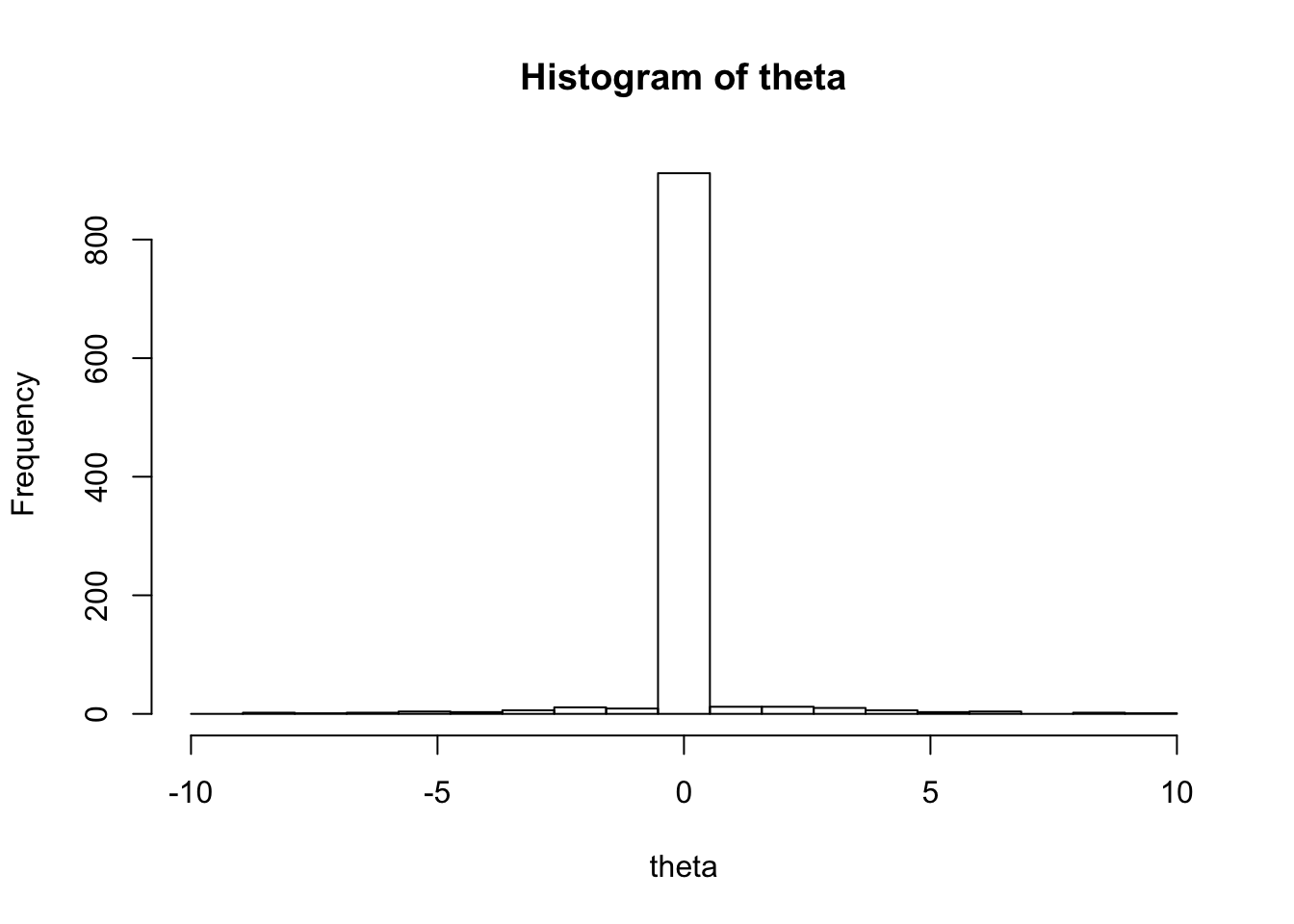
Now do inference under the EBNM model. Notice how the small values are shrunk hard, and the big values are hardly shrunk at all.
library("ashr")
library("ebnm")
x.pn = ebnm_point_normal(x,1)
plot(x,get_pm(x.pn),main="observation (x) vs posterior mean", ylab="posterior mean")
abline(a=0,b=1,col="red")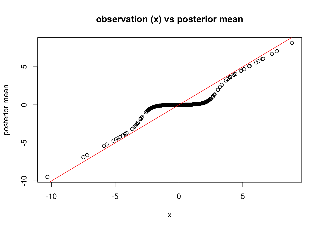
What about soft thresholding?
soft_thresh = function(x,lambda){
  ifelse(abs(x)>lambda, sign(x)*(abs(x)-lambda), 0)
}
plot(x,soft_thresh(x,1.5),main="observation (x) vs soft-thresholding estimate (lambda=1.5)",ylab="soft-thresholded estimate")
abline(a=0,b=1,col="red")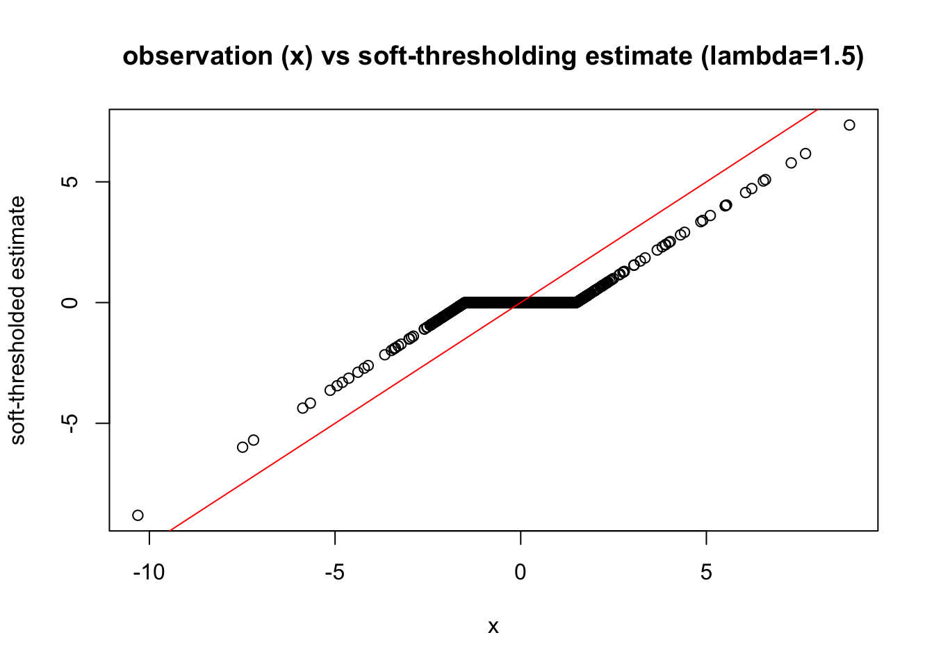
Now look at Mean Squared Error. Notice that both do much better than no shrinkage!!
mse = rep(0,100)
l = seq(0,5,length=100)
for(i in 1:100){
  mse[i] = mean((theta-soft_thresh(x,l[i]))^2)
}
plot(l,mse,ylim=c(0,1.2), main="black = no shrinkage; red=Empirical Bayes; points= soft-thresholding", xlab="lambda")
abline(h=mean((theta-get_pm(x.pn))^2),col="red")
abline(h=mean((theta-x)^2),col="blue")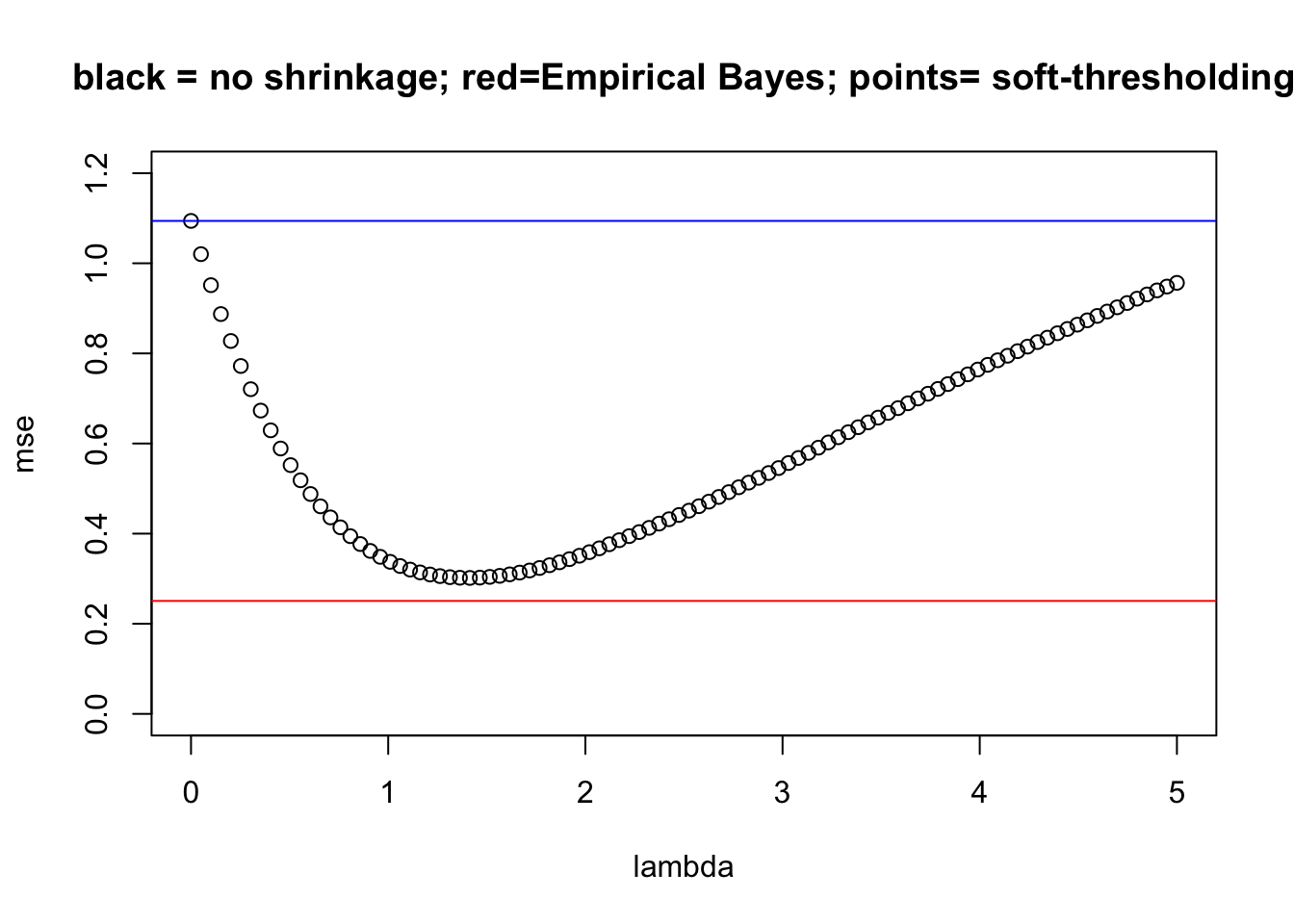
Session information
sessionInfo()R version 3.3.2 (2016-10-31)
Platform: x86_64-apple-darwin13.4.0 (64-bit)
Running under: OS X El Capitan 10.11.6
locale:
[1] en_US.UTF-8/en_US.UTF-8/en_US.UTF-8/C/en_US.UTF-8/en_US.UTF-8
attached base packages:
[1] stats graphics grDevices utils datasets methods base
other attached packages:
[1] ebnm_0.1-10 ashr_2.2-7
loaded via a namespace (and not attached):
[1] Rcpp_0.12.16 knitr_1.20 whisker_0.3-2
[4] magrittr_1.5 workflowr_1.0.1 MASS_7.3-49
[7] pscl_1.5.2 doParallel_1.0.11 SQUAREM_2017.10-1
[10] lattice_0.20-35 foreach_1.4.4 stringr_1.3.0
[13] tools_3.3.2 parallel_3.3.2 grid_3.3.2
[16] R.oo_1.22.0 git2r_0.21.0 htmltools_0.3.6
[19] iterators_1.0.9 yaml_2.1.18 rprojroot_1.3-2
[22] digest_0.6.15 Matrix_1.2-14 R.utils_2.6.0
[25] codetools_0.2-15 evaluate_0.10.1 rmarkdown_1.9
[28] stringi_1.1.7 backports_1.1.2 R.methodsS3_1.7.1
[31] truncnorm_1.0-7 This reproducible R Markdown analysis was created with workflowr 1.0.1