Cell cycle genes
Matthew Stephens
April 9, 2018
Last updated: 2018-05-21
workflowr checks: (Click a bullet for more information)-
✔ R Markdown file: up-to-date
Great! Since the R Markdown file has been committed to the Git repository, you know the exact version of the code that produced these results.
-
✔ Environment: empty
Great job! The global environment was empty. Objects defined in the global environment can affect the analysis in your R Markdown file in unknown ways. For reproduciblity it’s best to always run the code in an empty environment.
-
✔ Seed:
set.seed(20180411)The command
set.seed(20180411)was run prior to running the code in the R Markdown file. Setting a seed ensures that any results that rely on randomness, e.g. subsampling or permutations, are reproducible. -
✔ Session information: recorded
Great job! Recording the operating system, R version, and package versions is critical for reproducibility.
-
Great! You are using Git for version control. Tracking code development and connecting the code version to the results is critical for reproducibility. The version displayed above was the version of the Git repository at the time these results were generated.✔ Repository version: d63b9eb
Note that you need to be careful to ensure that all relevant files for the analysis have been committed to Git prior to generating the results (you can usewflow_publishorwflow_git_commit). workflowr only checks the R Markdown file, but you know if there are other scripts or data files that it depends on. Below is the status of the Git repository when the results were generated:
Note that any generated files, e.g. HTML, png, CSS, etc., are not included in this status report because it is ok for generated content to have uncommitted changes.Ignored files: Ignored: .DS_Store Ignored: .Rhistory Ignored: .Rproj.user/ Ignored: .sos/ Ignored: exams/ Ignored: temp/ Untracked files: Untracked: analysis/neanderthal.Rmd Untracked: analysis/pca_cell_cycle.Rmd Untracked: analysis/ridge_mle.Rmd Untracked: data/reduced.chr12.90-100.data.txt Untracked: data/reduced.chr12.90-100.snp.txt Untracked: docs/figure/pca_cell_cycle.Rmd/ Untracked: homework/fdr.aux Untracked: homework/fdr.log Untracked: tempETA_1_parBayesC.dat Untracked: temp_ETA_1_parBayesC.dat Untracked: temp_mu.dat Untracked: temp_varE.dat Untracked: tempmu.dat Untracked: tempvarE.dat Unstaged changes: Modified: analysis/eb_vs_soft.Rmd
Expand here to see past versions:
| File | Version | Author | Date | Message |
|---|---|---|---|---|
| Rmd | d63b9eb | stephens999 | 2018-05-21 | workflowr::wflow_publish(“svd_zip.Rmd”) |
| Rmd | 3d82c11 | stephens999 | 2018-04-11 | update cell cycle example to include circularity of trend filtering |
| Rmd | 463d7d9 | stephens999 | 2018-04-11 | update to include trend filter |
| Rmd | 8b80a72 | stephens999 | 2018-04-09 | add cell cycle example |
Some Cell Cycle Data
The data come from a recent experiment performed in the Gilad lab by Po Tung, in collaboration with Joyce Hsiao and others.
Since this is an anlaysis in progress, there is a lot we do not know about these data.
The data are measuring the activity of 10 genes that may or may not be involved in the “cell cycle”, which is the process cells go through as they divide. (We have data on a large number of genes, but Joyce has picked out 10 of them for us to look at.) Each gene is measured in many single cells, and we have some independent (but noisy) measurement of where each cell is in the cell cycle.
d = readRDS("../data/cyclegenes.rds")
dim(d)
[1] 990 11Here each row is a single cell. The first column (“theta”) is an estimate of where that cell is in the cell cycle, from 0 to 2pi. (Note that we don’t know what stage of the cell cycle each point in the interval corresponds to - so there is no guarantee that 0 is the “start” of the cell cycle. Also, because of the way these data were created we don’t know which direction the cell cycle is going - it could be forward or backward.) Then there are 10 columns corresponding to 10 different genes.
I’m going to order the rows by cell cycle (theta, first column) as this will make things much easier later.
# order the data
o = order(d[,1])
d = d[o,]
plot(d$theta)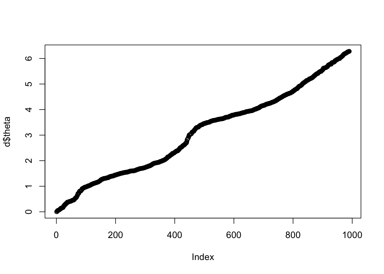
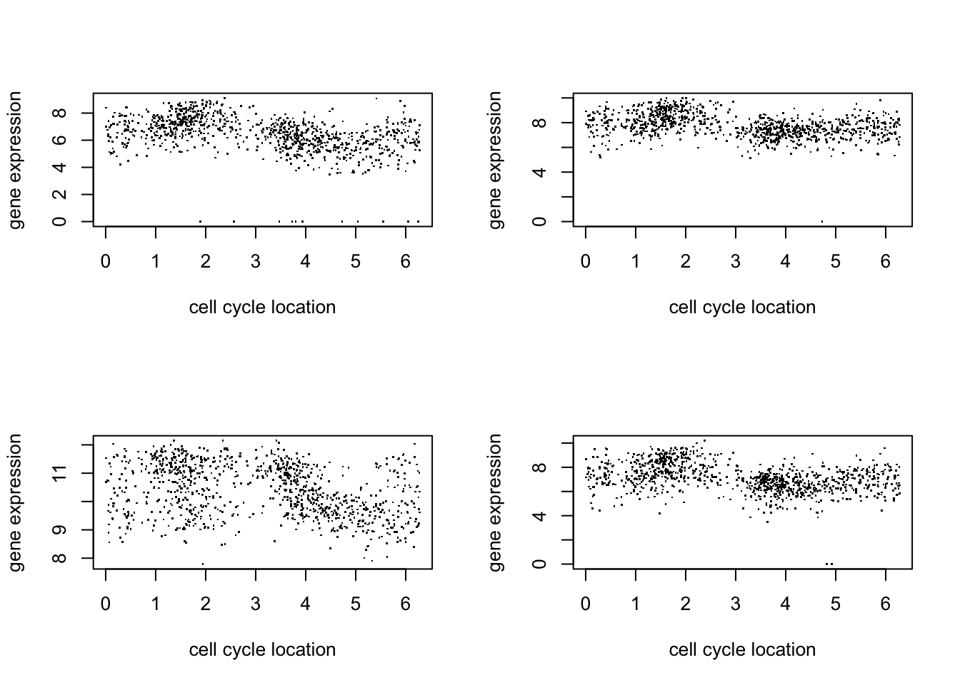
Here we just plot 8 genes to get a sense for the data:
par(mfcol=c(2,2))
for(i in 1:4){
  plot(d$theta, d[,(i+1)],pch=".",ylab="gene expression",xlab="cell cycle location")
}
par(mfcol=c(2,2))
for(i in 1:4){
  plot(d$theta, d[,(i+5)],pch=".",ylab="gene expression",xlab="cell cycle location")
}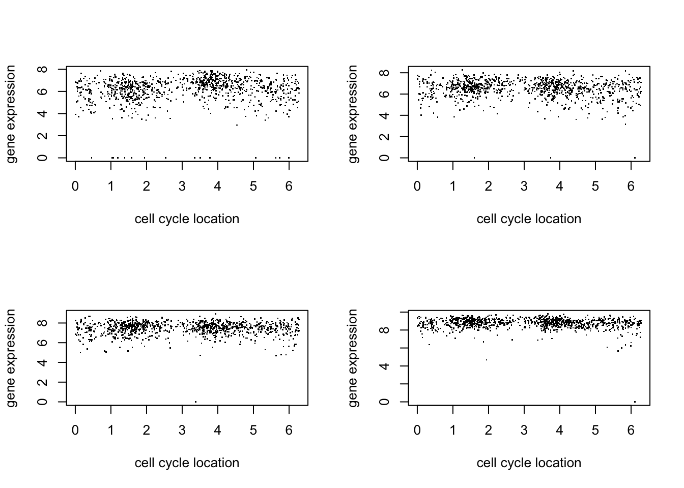
The question we want to answer is this: which genes show greatest evidence for varying in their expression through the cell cycle? For now what we really want is a filter we can apply to a large number of genes to pick out the ones that look most “interesting”. Later we might want a more formal statistical measure of evidence.
Our current idea is to try “smoothing” these data, and pick out genes where the change in the mean over theta is most variable (in some sense). The extreme would be if the smoother fits a horizontal line - that indicates no variability with theta, so those genes are not interesting to us.
Trend filtering
Here we will apply trend filtering to smooth these data. Trend filtering, at its simplest, applies L1 regularization to the changes in mean from one observation to the next. (The extreme would be no changes in any of these means, so a flat line.) It is implemented in the “genlasso” package.
library(genlasso)Loading required package: MASSLoading required package: MatrixLoading required package: igraph
Attaching package: 'igraph'The following objects are masked from 'package:stats':
decompose, spectrumThe following object is masked from 'package:base':
uniond2.tf = trendfilter(d[,2],ord = 1)Warning: 'rBind' is deprecated.
Since R version 3.2.0, base's rbind() should work fine with S4 objectsd2.tf.cv = cv.trendfilter(d2.tf) # performs 5-fold CVFold 1 ... Fold 2 ... Fold 3 ... Fold 4 ... Fold 5 ... plot(d[,1],d[,2],xlab="cell cycle",ylab="expression")
lines(d[,1],predict(d2.tf, d2.tf.cv$lambda.min)$fit,col=2,lwd=3)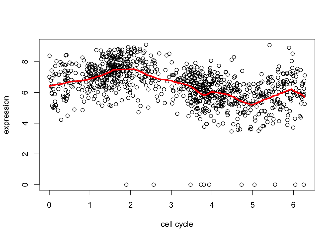
This fit is a bit on the “spiky” side in places. We can get a smoother fit by using a higher order filter. The details are too much to include here, but basically instead of shrinking first order differences it shrinks things that also measure differences with neighbors a bit further apart (2nd order).
d2.tf2 = trendfilter(d[,2],ord = 2)
d2.tf2.cv = cv.trendfilter(d2.tf2) # performs 5-fold CV
Fold 1 ... Fold 2 ... Fold 3 ... Fold 4 ... Fold 5 ... plot(d[,1],d[,2],xlab="cell cycle",ylab="expression")
lines(d[,1],predict(d2.tf, d2.tf.cv$lambda.min)$fit,col=2,lwd=3)
lines(d[,1],predict(d2.tf2, d2.tf2.cv$lambda.min)$fit,col=3,lwd=3)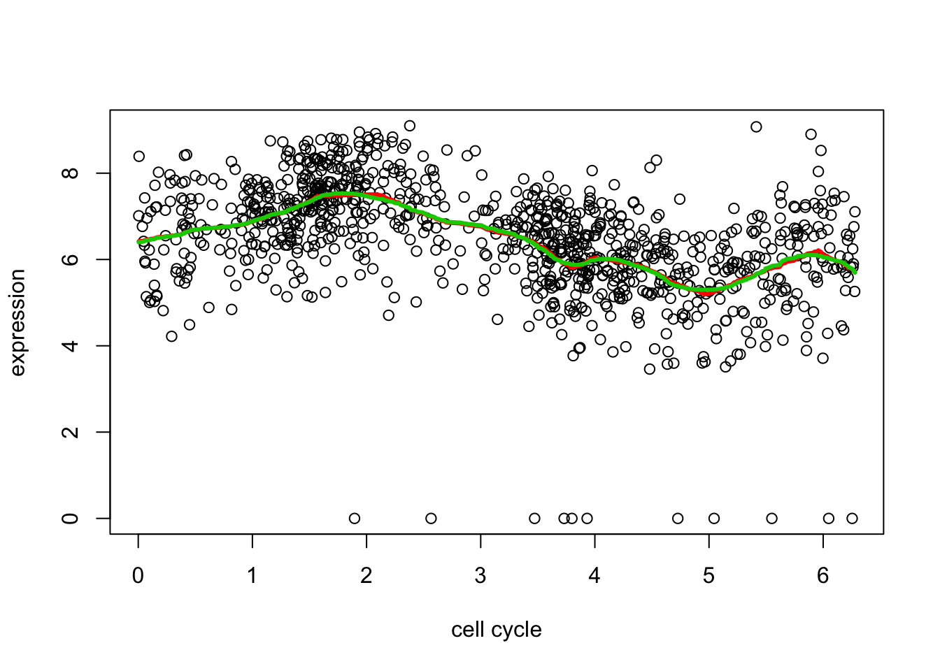
And here we try another gene that maybe shows less evidence for variability.
d7.tf2 = trendfilter(d[,7],ord = 2)
d7.tf2.cv = cv.trendfilter(d7.tf2) # performs 5-fold CV
Fold 1 ... Fold 2 ... Fold 3 ... Fold 4 ... Fold 5 ... plot(d[,1],d[,7],xlab="cell cycle",ylab="expression")
lines(d[,1],predict(d7.tf2, d7.tf2.cv$lambda.min)$fit,col=3,lwd=3)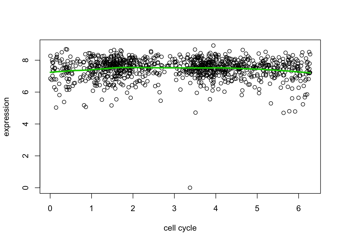
Dealing with the circularity
Because the \(x\) axis here is cyclical, the value of \(E(Y|x)\) near \(x=0\) should be similar to the value near \(x=2pi\). But trend filtering does not know this. We can encourage this behaviour by duplicating the data using a translation. (Note this is different than reflecting it about the boundaries).
Here is an example:
yy = c(d[,2],d[,2],d[,2]) ## duplicated data
xx = c(d[,1]-2*pi, d[,1], d[,1]+2*pi) # shifted/translated x coordinates

yy.tf2 = trendfilter(yy,ord = 2)
yy.tf2.cv = cv.trendfilter(yy.tf2) # performs 5-fold CV
Fold 1 ... Fold 2 ... Fold 3 ... Fold 4 ... Fold 5 ... plot(xx,yy,xlab="cell cycle",ylab="expression")
lines(xx,predict(yy.tf2, yy.tf2.cv$lambda.min)$fit,col=3,lwd=3)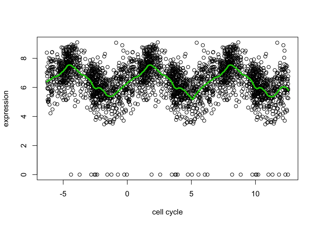
# plot only a single version of data
include = c(rep(FALSE,length(d[,2])), rep(TRUE, length(d[,2])), rep(FALSE, length(d[,2])))
plot(xx[include],yy[include],xlab="cell cycle",ylab="expression", main="trend filtering with circular fit")
lines(xx[include],predict(yy.tf2, yy.tf2.cv$lambda.min)$fit[include],col=3,lwd=3)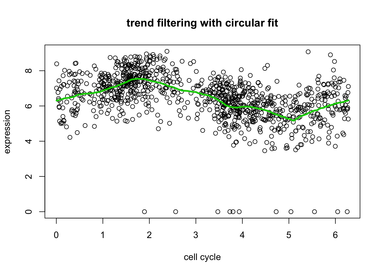
Wavelets
Here we will apply wavelets to smooth these data.
To apply wavelets we need the data to be a power of 2. Also we need the data to be ordered in terms of theta. We’ll subset the data to 512 elements here, and order it:
# subset the data
set.seed(1)
subset = sort(sample(1:nrow(d),512,replace=FALSE))
d.sub = d[subset,]
Here we do the Haar wavelet by specifying family="DaubExPhase",filter.number = 1 to the discrete wavelet transform function wd. The plot shows the wavelet transformed values, separately at each resolution.
library("wavethresh")WaveThresh: R wavelet software, release 4.6.8, installedCopyright Guy Nason and others 1993-2016Note: nlevels has been renamed to nlevelsWTwds <- wd(d.sub[,2],family="DaubExPhase",filter.number = 1)
plot(wds)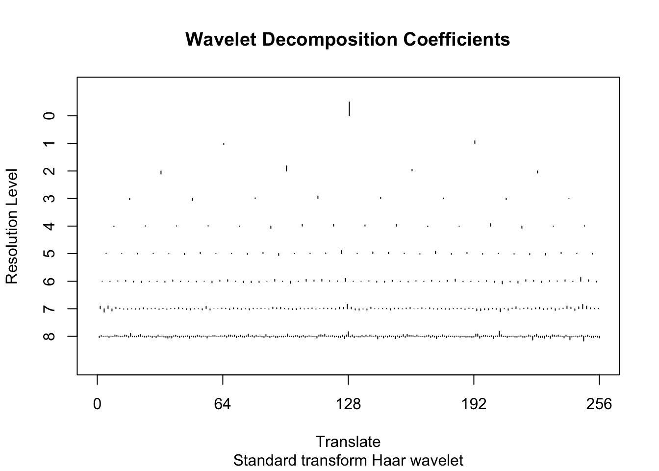
[1] 12.1009 12.1009 12.1009 12.1009 12.1009 12.1009 12.1009 12.1009 12.1009To illustrate the idea behind wavelet shrinkage we use the policy “manual” to shrink all the high-resolution coefficients (levels 4-8) to 0.
wtd <- threshold(wds, levels = 4:8,  policy="manual",value = 99999)
plot(wtd) 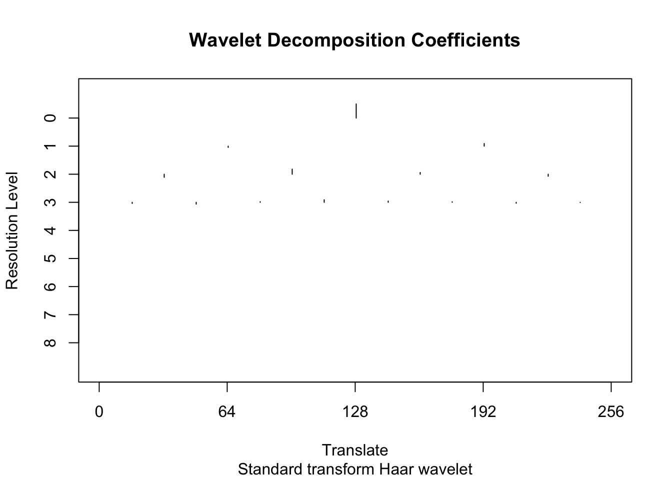
[1] 12.1009 12.1009 12.1009 12.1009 12.1009 12.1009 12.1009 12.1009 12.1009Now undo the wavelet transform on the shrunken coefficients
fd <- wr(wtd) #reconstruct
plot(d.sub$theta,d.sub[,2],xlab="cell cycle", ylab = "Expression")
lines(d.sub$theta,fd,col=2,lwd=3)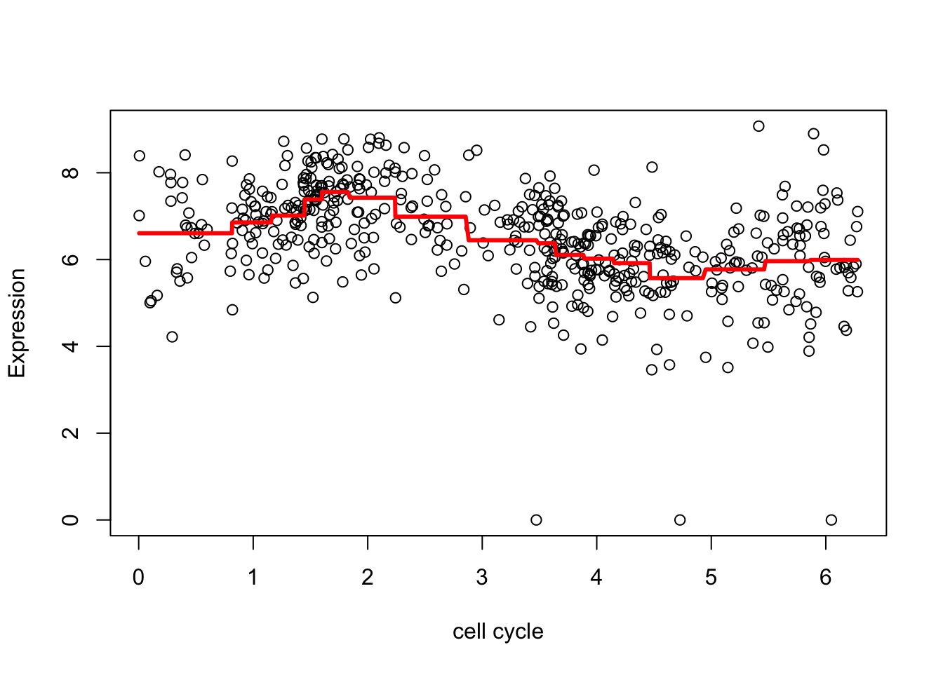
The estimate here is a bit “jumpy”, due to the use of the Haar wavelet and the rather naive hard thresholding. We can make it less “jumpy” by using a “less step-wise” wavelet basis
wds <- wd(d.sub[,2],family="DaubLeAsymm",filter.number = 8)
wtd <- threshold(wds, levels = 4:8,  policy="manual",value = 99999)
fd <- wr(wtd) #reconstruct
plot(d.sub$theta,d.sub[,2],xlab="cell cycle", ylab = "Expression")
lines(d.sub$theta,fd,col=2,lwd=3)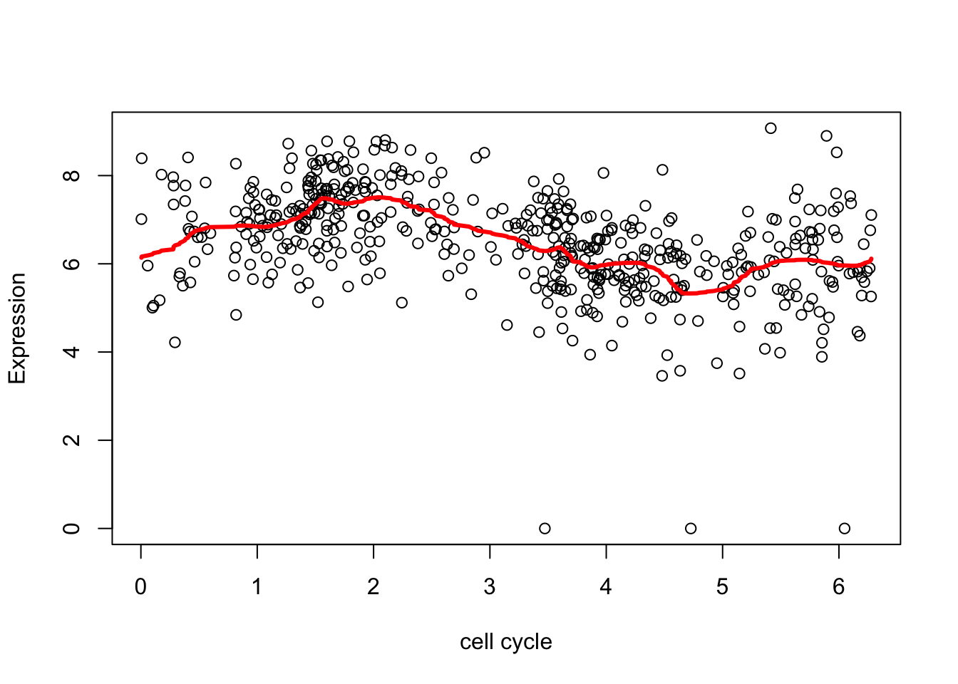
What happens if we use an Empirical Bayes thresholding rule?
The EbayesThresh package essentially solves the EBNM problem, using a prior distribution that is a mixture of a point mass at 0 and a Laplace distribution with rate parameter \(a\): \[ \pi_0 \delta_0 + (1-\pi_0) DExp(a).\]
Here a=NA tells Ebayesthresh ot estimate \(a\). Notice that the outliers cause “problems”
library("EbayesThresh")
wds <- wd(d.sub[,2],family="DaubLeAsymm",filter.number = 8)
wtd <- ebayesthresh.wavelet(wds,a=NA)
fd <- wr(wtd) #reconstruct
plot(d.sub$theta,d.sub[,2],xlab="cell cycle", ylab = "Expression")
lines(d.sub$theta,fd,col=2,lwd=3)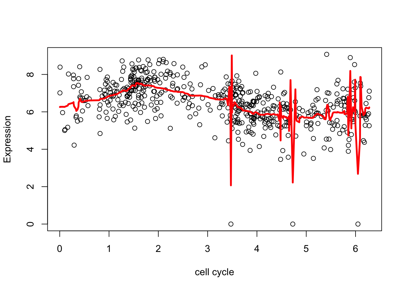
Try removing the outliers (actually setting them to the mean here), just to see what happens.
xx = ifelse(d.sub[,2]<2,mean(d.sub[,2]),d.sub[,2])
wds <- wd(xx,family="DaubLeAsymm",filter.number = 8)
wtd <- ebayesthresh.wavelet(wds,a=NA)
fd <- wr(wtd) #reconstruct
plot(d.sub$theta,xx,xlab="cell cycle", ylab = "Expression")
lines(d.sub$theta,fd,col=2,lwd=3)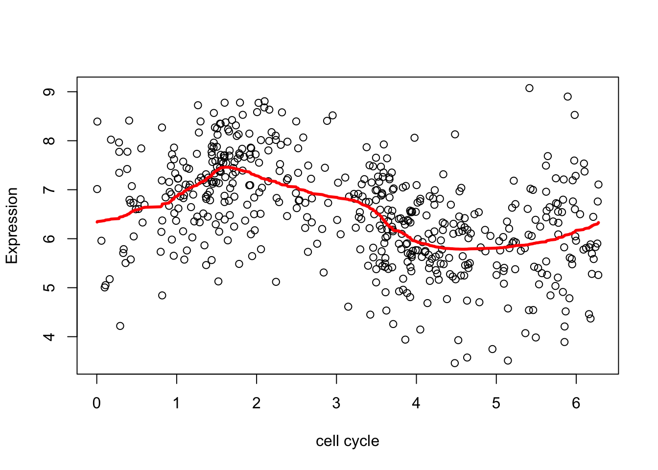
Notice that estimating \(a\) is really important (the default is to set \(a=0.5\)):
xx = ifelse(d.sub[,2]<2,mean(d.sub[,2]),d.sub[,2])
wds <- wd(xx,family="DaubLeAsymm",filter.number = 8)
wtd <- ebayesthresh.wavelet(wds)
fd <- wr(wtd) #reconstruct
plot(d.sub$theta,xx,xlab="cell cycle", ylab = "Expression")
lines(d.sub$theta,fd,col=2,lwd=3)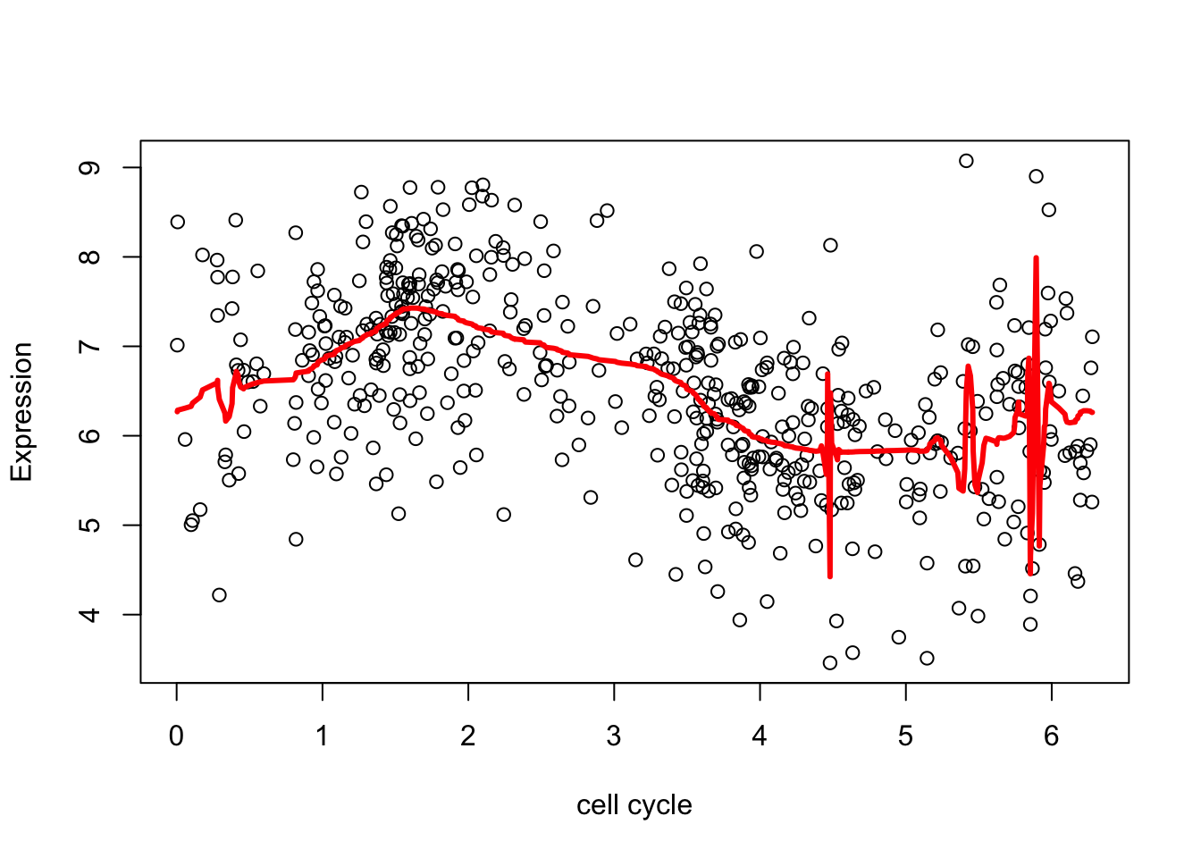
Dealing with the circularity
Note that the default in this particular package (wavethresh) is to assume the data are periodic on their region of definition - that is, circular. So we don’t have to do anything special here. It is taken care of!
Session information
sessionInfo()R version 3.3.2 (2016-10-31)
Platform: x86_64-apple-darwin13.4.0 (64-bit)
Running under: OS X El Capitan 10.11.6
locale:
[1] en_US.UTF-8/en_US.UTF-8/en_US.UTF-8/C/en_US.UTF-8/en_US.UTF-8
attached base packages:
[1] stats graphics grDevices utils datasets methods base
other attached packages:
[1] EbayesThresh_1.5-3 wavethresh_4.6.8 genlasso_1.3
[4] igraph_1.2.1 Matrix_1.2-14 MASS_7.3-49
loaded via a namespace (and not attached):
[1] Rcpp_0.12.16 knitr_1.20 whisker_0.3-2
[4] magrittr_1.5 workflowr_1.0.1 pscl_1.5.2
[7] doParallel_1.0.11 SQUAREM_2017.10-1 lattice_0.20-35
[10] foreach_1.4.4 ashr_2.2-7 stringr_1.3.0
[13] tools_3.3.2 parallel_3.3.2 grid_3.3.2
[16] R.oo_1.22.0 git2r_0.21.0 iterators_1.0.9
[19] htmltools_0.3.6 yaml_2.1.18 rprojroot_1.3-2
[22] digest_0.6.15 codetools_0.2-15 R.utils_2.6.0
[25] evaluate_0.10.1 rmarkdown_1.9 stringi_1.1.7
[28] backports_1.1.2 R.methodsS3_1.7.1 truncnorm_1.0-7
[31] pkgconfig_2.0.1 This reproducible R Markdown analysis was created with workflowr 1.0.1