Simple simulations for a simplified version of web-boost-2

Simulation of data

Run mr.ash

Run a simplified version of veb-boost (mr.ash2s)

start with gene
start with SNP

Last updated: 2020-06-10

Checks: 6 1

Knit directory: causal-TWAS/

This reproducible R Markdown analysis was created with workflowr (version 1.6.0). The Checks tab describes the reproducibility checks that were applied when the results were created. The Past versions tab lists the development history.

R Markdown file: up-to-date

Great! Since the R Markdown file has been committed to the Git repository, you know the exact version of the code that produced these results.

Environment: empty

Great job! The global environment was empty. Objects defined in the global environment can affect the analysis in your R Markdown file in unknown ways. For reproduciblity it’s best to always run the code in an empty environment.

Seed: set.seed(20191103)

The command set.seed(20191103) was run prior to running the code in the R Markdown file. Setting a seed ensures that any results that rely on randomness, e.g. subsampling or permutations, are reproducible.

Session information: recorded

Great job! Recording the operating system, R version, and package versions is critical for reproducibility.

Cache: none

Nice! There were no cached chunks for this analysis, so you can be confident that you successfully produced the results during this run.

File paths: absolute

Using absolute paths to the files within your workflowr project makes it difficult for you and others to run your code on a different machine. Change the absolute path(s) below to the suggested relative path(s) to make your code more reproducible.

absolute	relative
~/causalTWAS/causal-TWAS/code/fit_mr.ash.R	code/fit_mr.ash.R
~/causalTWAS/causal-TWAS/code/mr.ash2.R	code/mr.ash2.R

Repository version: 8f01adb

Great! You are using Git for version control. Tracking code development and connecting the code version to the results is critical for reproducibility. The version displayed above was the version of the Git repository at the time these results were generated.

Note that you need to be careful to ensure that all relevant files for the analysis have been committed to Git prior to generating the results (you can use wflow_publish or wflow_git_commit). workflowr only checks the R Markdown file, but you know if there are other scripts or data files that it depends on. Below is the status of the Git repository when the results were generated:


Ignored files:
    Ignored:    .Rhistory
    Ignored:    .Rproj.user/
    Ignored:    .ipynb_checkpoints/
    Ignored:    code/.ipynb_checkpoints/
    Ignored:    data/

Untracked files:
    Untracked:  code/gen_mr.ash2_output.R
    Untracked:  code/gwas.R
    Untracked:  code/run_gwas_expr.R
    Untracked:  code/run_gwas_snp.R

Unstaged changes:
    Modified:   analysis/simulation-simpleveb-boost-ukbchr22.Rmd
    Modified:   analysis/simulation-simpleveb-boost2-ukbchr22.Rmd
    Modified:   code/fit_mr.ash.R
    Modified:   code/mr.ash2.R
    Modified:   code/run_test_mr.ash2.R
    Modified:   code/run_test_susie.R
    Modified:   code/simulate_phenotype.R
    Modified:   code/temp.R
    Modified:   code/workflow-ashtest.ipynb
    Modified:   code/workflow-data.ipynb

Note that any generated files, e.g. HTML, png, CSS, etc., are not included in this status report because it is ok for generated content to have uncommitted changes.

These are the previous versions of the R Markdown and HTML files. If you’ve configured a remote Git repository (see ?wflow_git_remote), click on the hyperlinks in the table below to view them.

File	Version	Author	Date	Message
Rmd	8f01adb	simingz	2020-05-28	mr.ash2s
html	8f01adb	simingz	2020-05-28	mr.ash2s

Simulation of data

20 blocks:

Each block has either gene or SNP effect
Each block has 99 SNPs and 1 gene. Each gene is linear sum of the previous 3 SNPs.
Each block, either the gene or the last eQTL has non-zero effect on trait

The first 4 blocks have gene effect.

set.seed(1)
N <- 4000
nblocks <- 20
block.size <- 100
p <- nblocks * block.size
n.eQTL <- 3  # number of eQTLs per gene
sigma.eQTL <- 0.5 # eQTL effect size
sigma.SNP <- 0.1 # effect size of causal SNP on trait
sigma.gene <- 0.1 # effect size of causal gene on trait
X <- matrix(rep(0,0), nrow=N, ncol=0)
gamma.gene <- rep(0, nblocks) # indicator of genes
gamma.gene[1:4] <- 1 
beta <- numeric(0)
SNP.idx <- numeric(0)
for (i in 1:nblocks) {
  # sample SNP data
  X.block.SNP <- matrix(rnorm(N*(block.size-1)), nrow=N, ncol=block.size-1)
  SNP.idx <- c(SNP.idx, 1:(block.size-1) + (i-1)*block.size)
  
  # generate gene data: use the previous few SNPs as eQTL
  effects.eQTL <- rnorm(n.eQTL, 0, sigma.eQTL)
  X.block.gene <- X.block.SNP[, (block.size - n.eQTL):(block.size - 1)] %*% effects.eQTL
  X.block = cbind(X.block.SNP, X.block.gene)
  X <- cbind(X, X.block)
  
  # sample beta
  if (gamma.gene[i] == 1) { # gene effect in this block
    beta.SNP <- rep(0, block.size - 1)
    beta.gene <- rnorm(1, 0, sigma.gene)
  } else { # SNP effect in this block
    beta.SNP <- c(rep(0, block.size - 2), rnorm(1, 0, sigma.SNP))
    beta.gene <- 0
  }
  beta.block <- c(beta.SNP, beta.gene)
  beta <- c(beta, beta.block)
}
sigma.e <- 1
y <- X %*% beta + rnorm(N, 0, sigma.e)
gene.idx <- (1:nblocks) * block.size

Run mr.ash

summary_mr.ash <- function(fit){
  cat("pi1 = ", 1-fit$pi[[1]], "\n")
  pve <- get_pve(fit)
  cat("pve : ", pve, "\n")
}

plot_beta <- function(beta,beta.pm, ...){
  plot( beta, pch=19, col ="darkgreen", ...)
  points(beta.pm, pch =19, col = "red")
  legend("topright", legend=c("true beta", "posterior mean"),
       col=c("darkgreen", "red"), pch=19)
}

fit <- mr.ash(X, y, method="caisa")
summary_mr.ash(fit)

pi1 =  0.01126046 
pve :  0.1521592

plot_beta(beta[gene.idx], fit$beta[gene.idx], main = "beta for gene effect")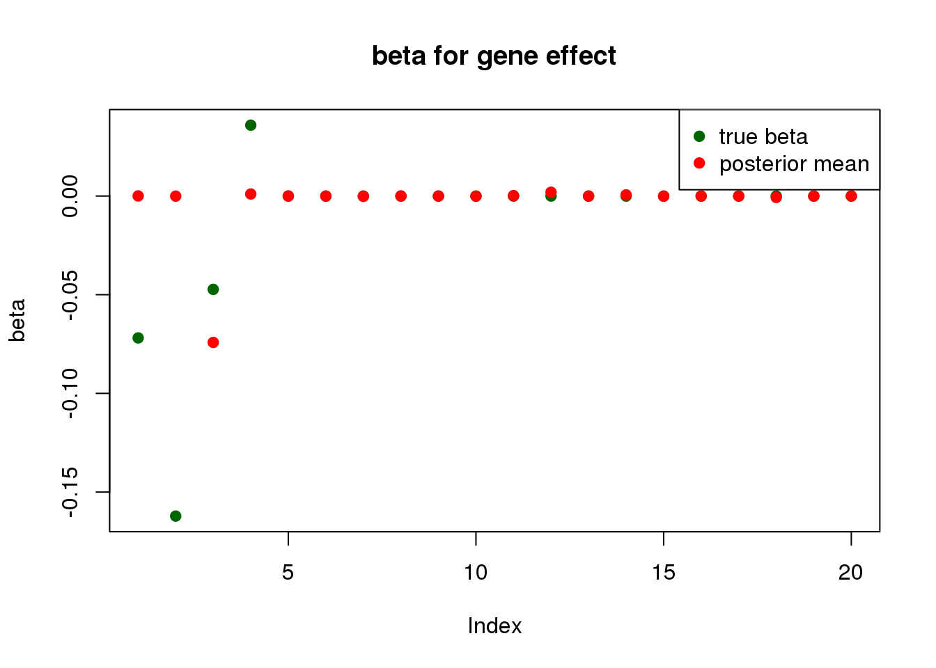

Version	Author	Date
8f01adb	simingz	2020-05-28

plot_beta(beta[SNP.idx], fit$beta[SNP.idx], main = "beta for SNP effect")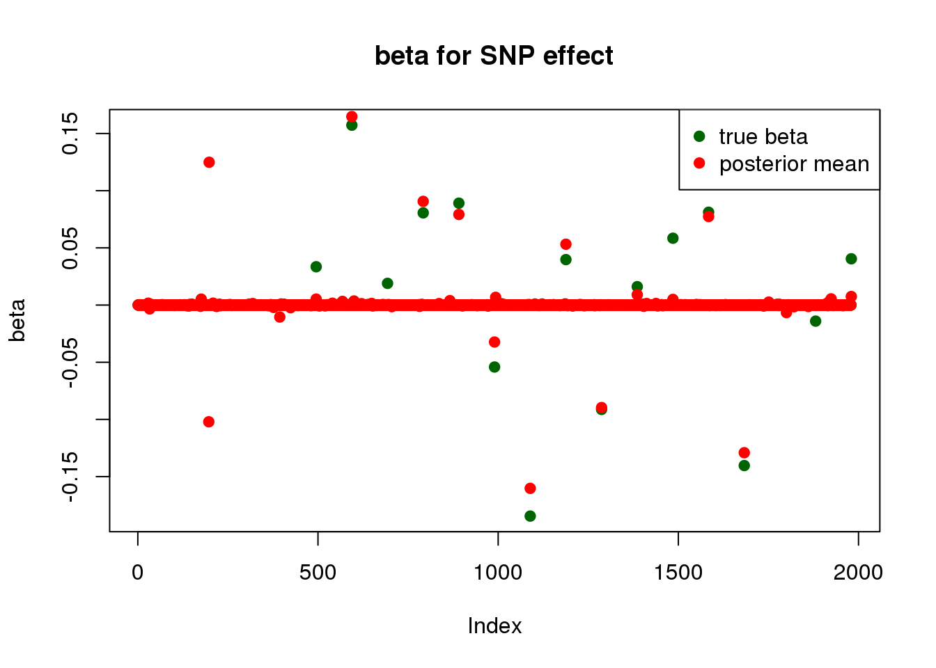

Version	Author	Date
8f01adb	simingz	2020-05-28

Run a simplified version of veb-boost (mr.ash2s)

start with gene

X.gene <- X[,gene.idx]
X.SNP <- X[, SNP.idx]
fit <- mr.ash2s(X.gene, X.SNP, y)

print("for gene effect: ")

[1] "for gene effect: "

summary_mr.ash(fit$fit1)

pi1 =  0.7510055 
pve :  0.03234752

plot_beta(beta[gene.idx], fit$fit1$beta, main = "beta for gene effect")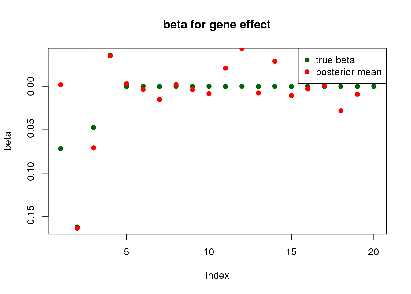

Version	Author	Date
8f01adb	simingz	2020-05-28

print("for SNP effect: ")

[1] "for SNP effect: "

summary_mr.ash(fit$fit2)

pi1 =  0.006990563 
pve :  0.1326746

plot_beta(beta[SNP.idx], fit$fit2$beta, main = "beta for SNP effect")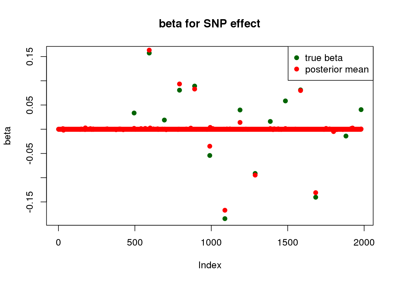

Version	Author	Date
8f01adb	simingz	2020-05-28

start with SNP

X.gene <- X[,gene.idx]
X.SNP <- X[, SNP.idx]
fit <- mr.ash2s(X.SNP, X.gene, y)

print("for gene effect: ")

[1] "for gene effect: "

summary_mr.ash(fit$fit2)

pi1 =  0.9149261 
pve :  0.01660308

plot_beta(beta[gene.idx], fit$fit2$beta, main = "beta for gene effect")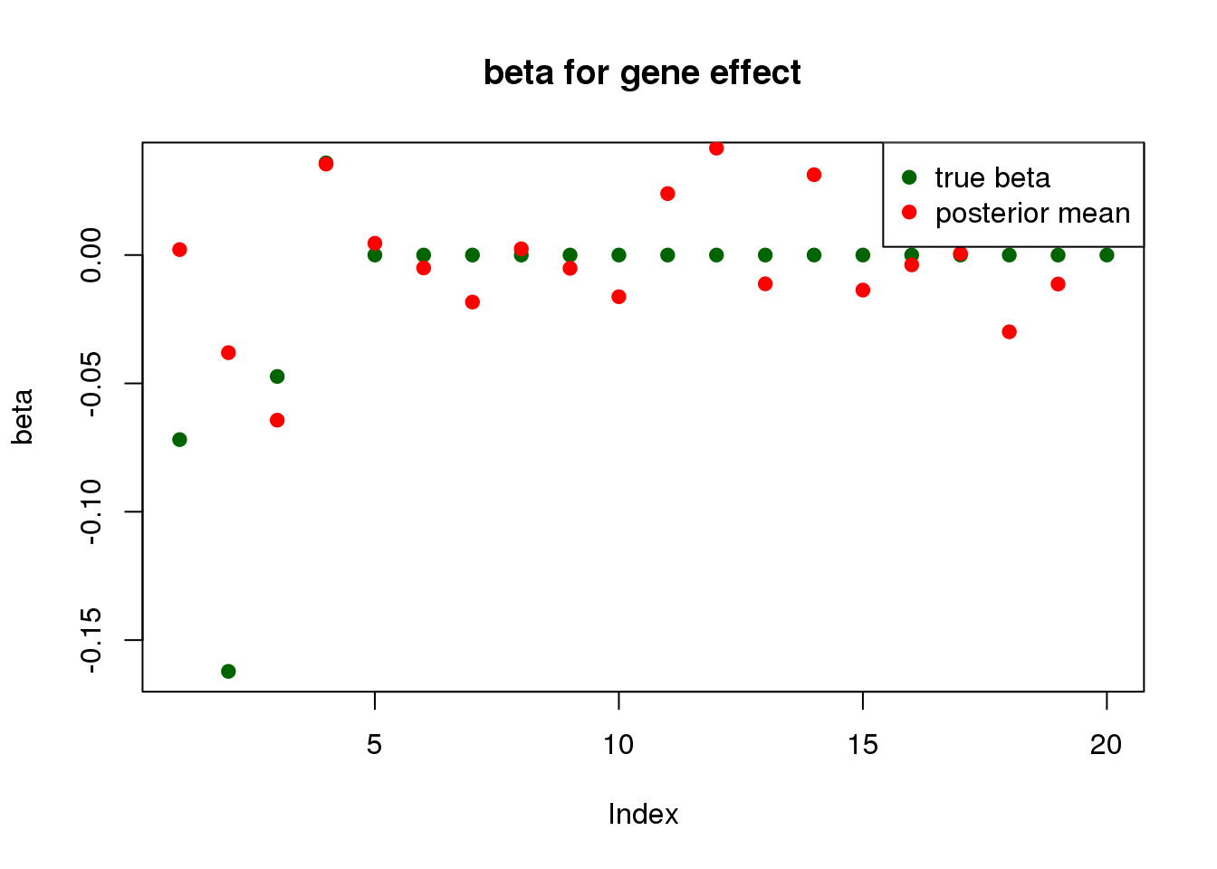

Version	Author	Date
8f01adb	simingz	2020-05-28

print("for SNP effect: ")

[1] "for SNP effect: "

summary_mr.ash(fit$fit1)

pi1 =  0.009254532 
pve :  0.1485855

plot_beta(beta[SNP.idx], fit$fit1$beta, main = "beta for SNP effect")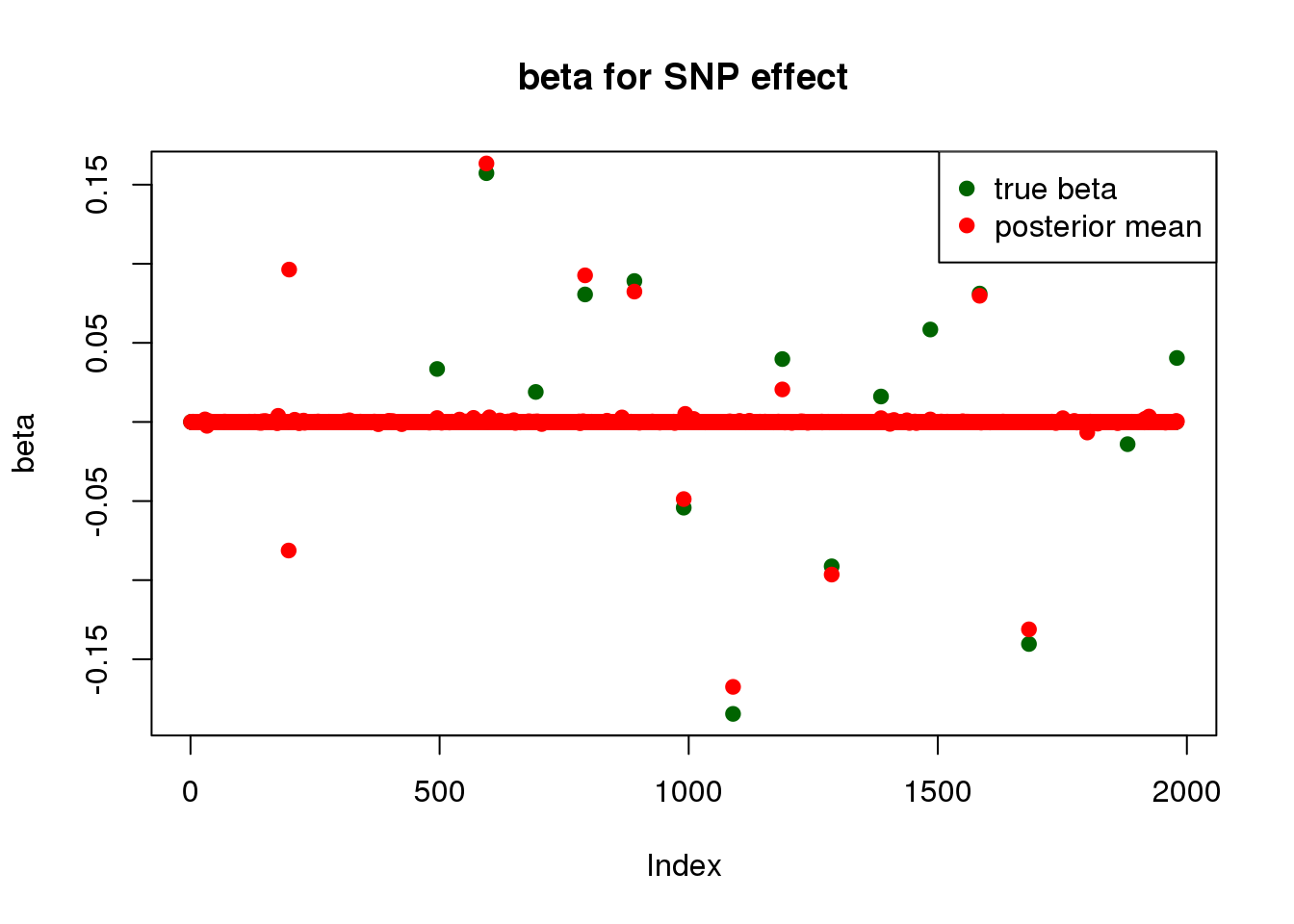

Version	Author	Date
8f01adb	simingz	2020-05-28

sessionInfo()

R version 3.5.1 (2018-07-02)
Platform: x86_64-pc-linux-gnu (64-bit)
Running under: Scientific Linux 7.4 (Nitrogen)

Matrix products: default
BLAS/LAPACK: /software/openblas-0.2.19-el7-x86_64/lib/libopenblas_haswellp-r0.2.19.so

locale:
 [1] LC_CTYPE=en_US.UTF-8       LC_NUMERIC=C              
 [3] LC_TIME=en_US.UTF-8        LC_COLLATE=en_US.UTF-8    
 [5] LC_MONETARY=en_US.UTF-8    LC_MESSAGES=en_US.UTF-8   
 [7] LC_PAPER=en_US.UTF-8       LC_NAME=C                 
 [9] LC_ADDRESS=C               LC_TELEPHONE=C            
[11] LC_MEASUREMENT=en_US.UTF-8 LC_IDENTIFICATION=C       

attached base packages:
[1] stats     graphics  grDevices utils     datasets  methods   base     

other attached packages:
[1] mr.ash.alpha_0.1-7

loaded via a namespace (and not attached):
 [1] workflowr_1.6.0 Rcpp_1.0.4.6    lattice_0.20-38 digest_0.6.25  
 [5] later_0.7.5     rprojroot_1.3-2 grid_3.5.1      R6_2.3.0       
 [9] backports_1.1.2 git2r_0.26.1    magrittr_1.5    evaluate_0.12  
[13] highr_0.7       stringi_1.3.1   fs_1.3.1        promises_1.0.1 
[17] whisker_0.3-2   Matrix_1.2-15   rmarkdown_1.10  tools_3.5.1    
[21] stringr_1.4.0   glue_1.4.1      httpuv_1.4.5    yaml_2.2.0     
[25] compiler_3.5.1  htmltools_0.3.6 knitr_1.20