Test a simpler version of veb-boost performance on ukbiobank data-2
Last updated: 2020-05-28
Checks: 5 2
Knit directory: causal-TWAS/
This reproducible R Markdown analysis was created with workflowr (version 1.6.0). The Checks tab describes the reproducibility checks that were applied when the results were created. The Past versions tab lists the development history.
The R Markdown is untracked by Git. To know which version of the R Markdown file created these results, you’ll want to first commit it to the Git repo. If you’re still working on the analysis, you can ignore this warning. When you’re finished, you can run wflow_publish to commit the R Markdown file and build the HTML.
Great job! The global environment was empty. Objects defined in the global environment can affect the analysis in your R Markdown file in unknown ways. For reproduciblity it’s best to always run the code in an empty environment.
The command set.seed(20191103) was run prior to running the code in the R Markdown file. Setting a seed ensures that any results that rely on randomness, e.g. subsampling or permutations, are reproducible.
Great job! Recording the operating system, R version, and package versions is critical for reproducibility.
Nice! There were no cached chunks for this analysis, so you can be confident that you successfully produced the results during this run.
Using absolute paths to the files within your workflowr project makes it difficult for you and others to run your code on a different machine. Change the absolute path(s) below to the suggested relative path(s) to make your code more reproducible.
| absolute | relative |
|---|---|
| ~/causalTWAS/causal-TWAS/code/fit_mr.ash.R | code/fit_mr.ash.R |
Great! You are using Git for version control. Tracking code development and connecting the code version to the results is critical for reproducibility. The version displayed above was the version of the Git repository at the time these results were generated.
Note that you need to be careful to ensure that all relevant files for the analysis have been committed to Git prior to generating the results (you can use wflow_publish or wflow_git_commit). workflowr only checks the R Markdown file, but you know if there are other scripts or data files that it depends on. Below is the status of the Git repository when the results were generated:
Ignored files:
    Ignored:    .Rhistory
    Ignored:    .Rproj.user/
    Ignored:    .ipynb_checkpoints/
    Ignored:    code/.ipynb_checkpoints/
    Ignored:    data/

Untracked files:
    Untracked:  analysis/figure/
    Untracked:  analysis/simulation-simpleveb-boost2-ukbchr22.Rmd
    Untracked:  analysis/simulation_simpleveb-boost2.Rmd
    Untracked:  analysis/simulation_susie.Rmd
    Untracked:  code/run_test_mr.ash2s.R
    Untracked:  code/run_test_susie.R

Unstaged changes:
    Modified:   analysis/index.Rmd
    Modified:   analysis/simulation_simpleveb-boost.Rmd
    Modified:   code/mr.ash2.R
    Modified:   code/run_test_mr.ash2.R
    Modified:   code/workflow-ashtest.ipynb

Staged changes:
    Renamed1:   code/simple_vebboost.R
    Renamed2:   code/mr.ash2.R
    Renamed1:   code/run_test_veb-boost.R
    Renamed2:   code/run_test_mr.ash2.R
Note that any generated files, e.g. HTML, png, CSS, etc., are not included in this status report because it is ok for generated content to have uncommitted changes.
There are no past versions. Publish this analysis with wflow_publish() to start tracking its development.
library(mr.ash.alpha)
source("~/causalTWAS/causal-TWAS/code/fit_mr.ash.R")
summary_mr.ash <- function(fit){
cat("pi1 = ", 1-fit$pi[[1]], "\n")
pve <- get_pve(fit)
cat("pve = ", pve, "\n")
}
plot_beta <- function(beta,beta.pm, ...){
plot( beta, pch=19, col ="darkgreen", ...)
points(beta.pm, pch =19, col = "red")
legend("topright", legend=c("true beta", "posterior mean"),
col=c("darkgreen", "red"), pch=19)
}
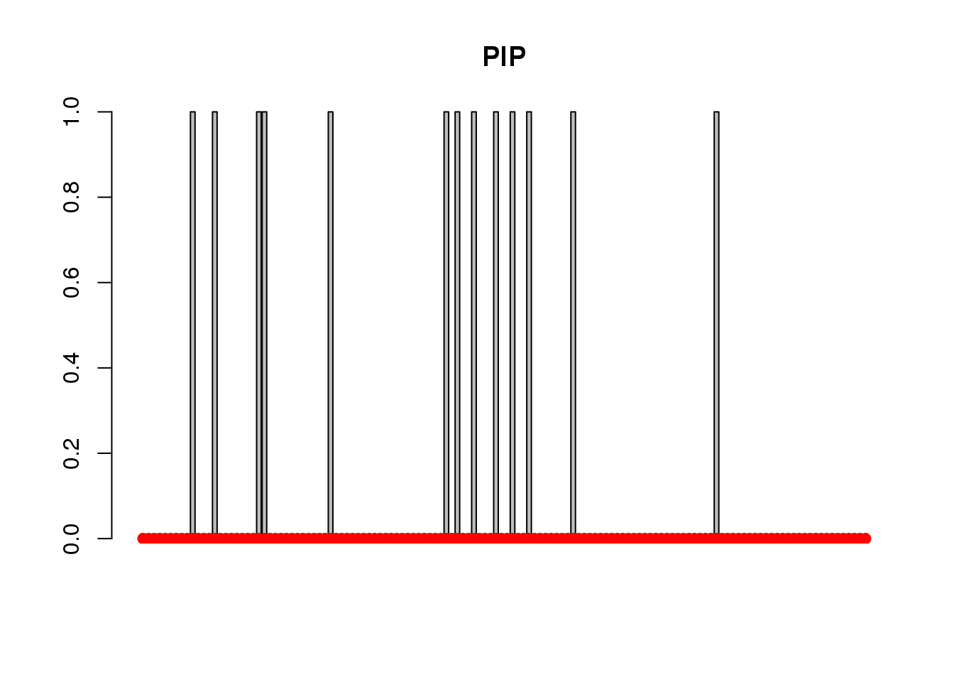
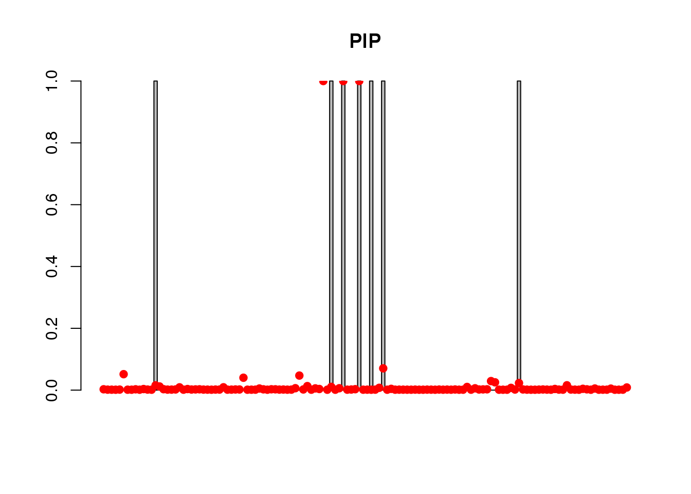
plot_pip <- function(indi, pip, pipcut = 0.1) {
x <- barplot(indi, main = "PIP")
points(x, pip, pch=19, col="red")
pred <- which(pip > pipcut)
real <- which(indi==1)
tp <- length(intersect(pred, real))/length(pred)
fp <- 1 - tp
fn <- length(setdiff(real, pred))/length(real)
cat("false positive rate: ", fp, "\n")
cat("false negative rate: ", fn, "\n")
}
summary_mr.ash2 <- function(g.fit, s.fit, phenores, pipcut = 0.1){
e.b <- rep(0, length(g.fit$beta))
e.b[phenores$param$idx.cgene] <- phenores$param$e.beta
cat("gene expression effect: \n")
summary_mr.ash(g.fit)
plot_beta(e.b, g.fit$beta)
indi <- rep(0, length(g.fit$beta))
indi[phenores$param$idx.cgene] <- 1
pip <- get_pip(g.fit)
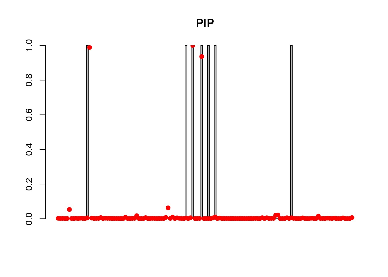
plot_pip(indi, pip, pipcut = pipcut)
s.b <- rep(0, length(s.fit$beta))
s.b[phenores$param$idx.cSNP] <- phenores$param$s.theta
cat("snp effect: \n")
summary_mr.ash(s.fit)
plot_beta(s.b, s.fit$beta)
}simdatadir <- "~/causalTWAS/simulations/simulation_ashtest_20200503/"
outputdir <- "~/causalTWAS/simulations/simulation_ashtest_20200527/"Simulation 1
True parameters:
load(paste0(simdatadir, "mr.ash2_20200503-1-pheno.Rd"))
readLines(paste0(simdatadir, "param-20200503-1.R"))
[1] "pve.expr <- 0.01" "pve.snp <- 0.05" "pi_beta <- 0.1"
[4] "pi_theta <- 1e-3" "tau <- 1" MR.ASH2s results (start from gene):
load(paste0(outputdir, "20200527-1-mr.ash2s.expr-res.Rd"))
g.fit <- mr.ash2s.fit$fit1
s.fit <- mr.ash2s.fit$fit2
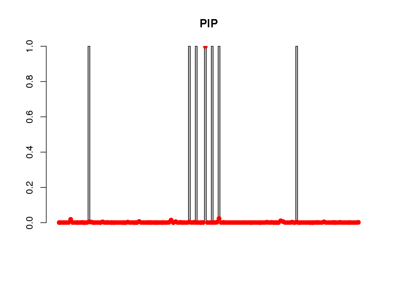
summary_mr.ash2(g.fit, s.fit, phenores)gene expression effect:
pi1 = 0.05417903
pve = 0.1336998 
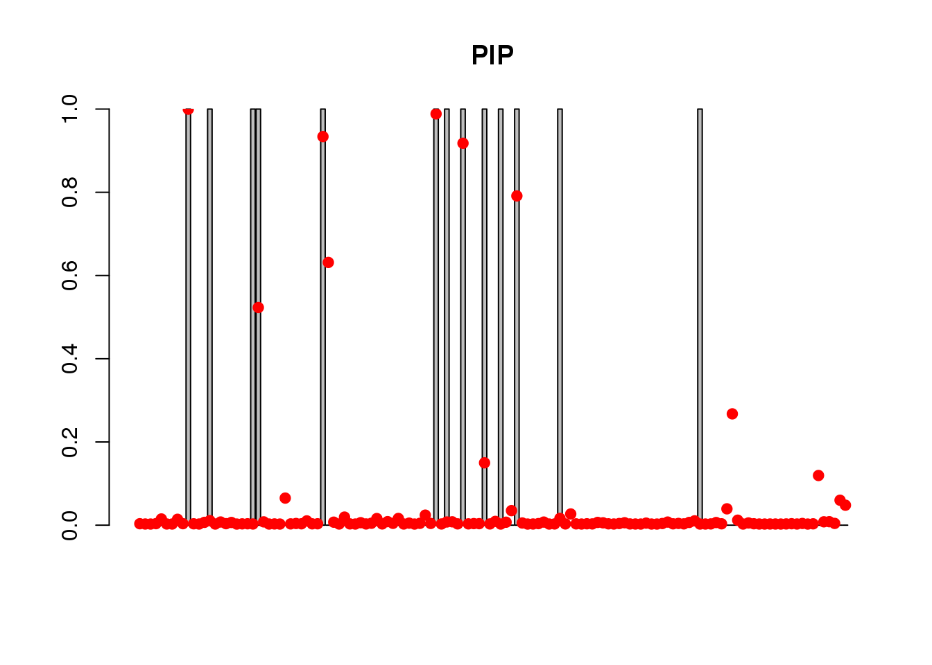
false positive rate:  0.3
false negative rate:  0.4615385
snp effect:
pi1 =  0.0001887495
pve = 0.2500488 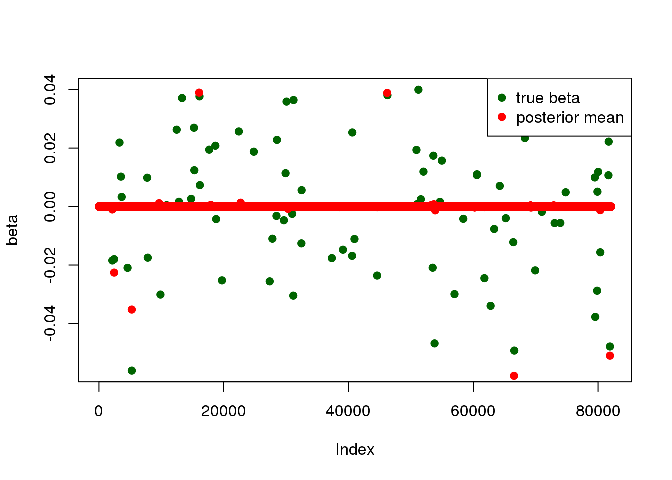
MR.ASH results (start from SNP):
load(paste0(outputdir, "20200527-1-mr.ash2s.snp-res.Rd"))
g.fit <- mr.ash2s.fit$fit2
s.fit <-  mr.ash2s.fit$fit1
summary_mr.ash2(g.fit, s.fit, phenores)
gene expression effect:
pi1 = 0.05417931
pve = 0.1337004 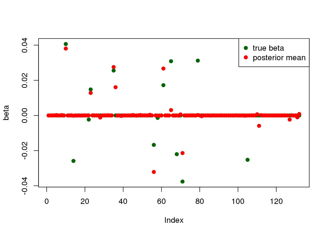

false positive rate:  0.3
false negative rate:  0.4615385
snp effect:
pi1 =  0.0001887502
pve = 0.2500495 
Simulation 2
True parameters:
load(paste0(simdatadir, "mr.ash2_20200503-2-pheno.Rd"))
readLines(paste0(simdatadir, "param-20200503-2.R"))
[1] "pve.expr <- 0.005" "pve.snp <- 0.01" "pi_beta <- 0.1"
[4] "pi_theta <- 1e-3" "tau <- 1" MR.ASH results (start from gene):
load(paste0(outputdir, "20200527-2-mr.ash2s.expr-res.Rd"))
g.fit <- mr.ash2s.fit$fit1
s.fit <-  mr.ash2s.fit$fit2
summary_mr.ash2(g.fit, s.fit, phenores)
gene expression effect:
pi1 = 1.973726e-10
pve = 7.959401e-08 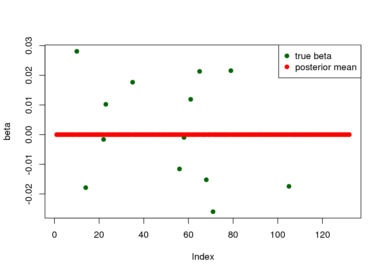
false positive rate:  NaN
false negative rate:  1
snp effect:
pi1 =  1.115821e-07
pve = 0.0002921814 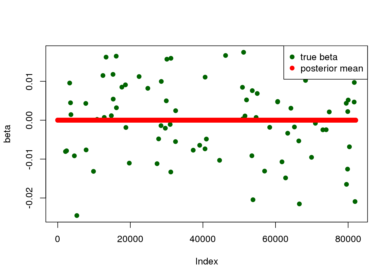
MR.ASH results (start from SNP):
load(paste0(outputdir, "20200527-2-mr.ash2s.snp-res.Rd"))
g.fit <- mr.ash2s.fit$fit2
s.fit <-  mr.ash2s.fit$fit1
summary_mr.ash2(g.fit, s.fit, phenores)
gene expression effect:
pi1 = 1.966005e-10
pve = 7.958468e-08 

false positive rate:  NaN
false negative rate:  1
snp effect:
pi1 =  1.196675e-07
pve = 0.0003063728 
Simulation 3
True parameters:
load(paste0(simdatadir, "mr.ash2_20200503-3-pheno.Rd"))
readLines(paste0(simdatadir, "param-20200503-3.R"))
[1] "pve.expr <- 0.01" "pve.snp <- 0.05" "pi_beta <- 0.05"
[4] "pi_theta <- 1e-4" "tau <- 1" MR.ASH results (start from gene):
load(paste0(outputdir, "20200527-3-mr.ash2s.expr-res.Rd"))
g.fit <- mr.ash2s.fit$fit1
s.fit <-  mr.ash2s.fit$fit2
summary_mr.ash2(g.fit, s.fit, phenores)
gene expression effect:
pi1 = 0.02753678
pve = 0.07367684 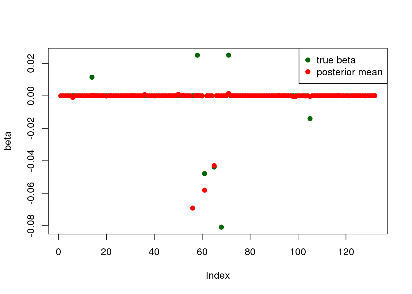
false positive rate:  0.3333333
false negative rate:  0.7142857
snp effect:
pi1 =  0.0001530549
pve = 0.2156009 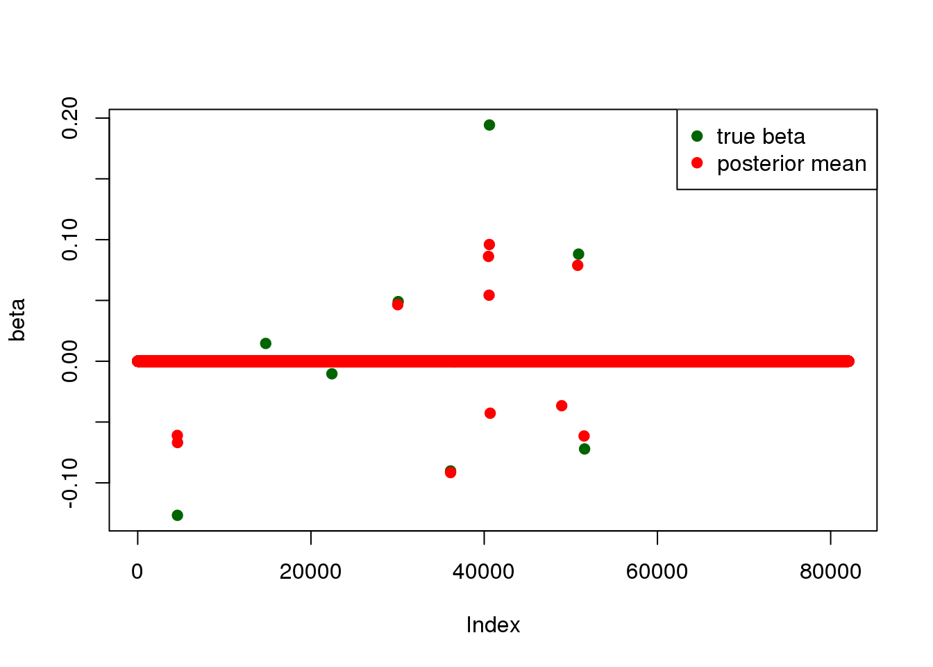
MR.ASH results (start from SNP):
load(paste0(outputdir, "20200527-3-mr.ash2s.snp-res.Rd"))
g.fit <- mr.ash2s.fit$fit2
s.fit <-  mr.ash2s.fit$fit1
summary_mr.ash2(g.fit, s.fit, phenores)
gene expression effect:
pi1 = 0.009105761
pve = 0.02562701 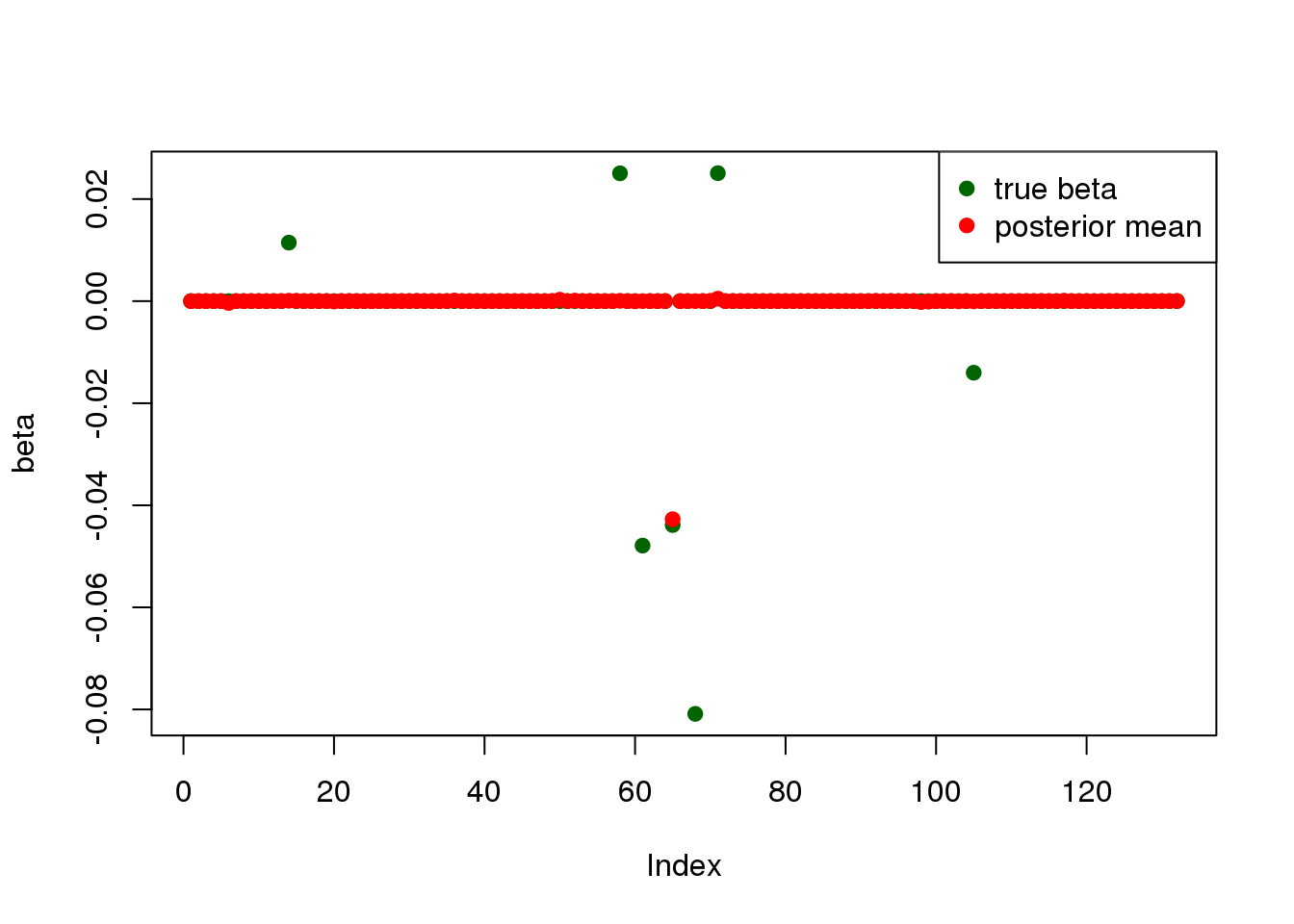
false positive rate:  0
false negative rate:  0.8571429
snp effect:
pi1 =  0.0001684206
pve = 0.2321756 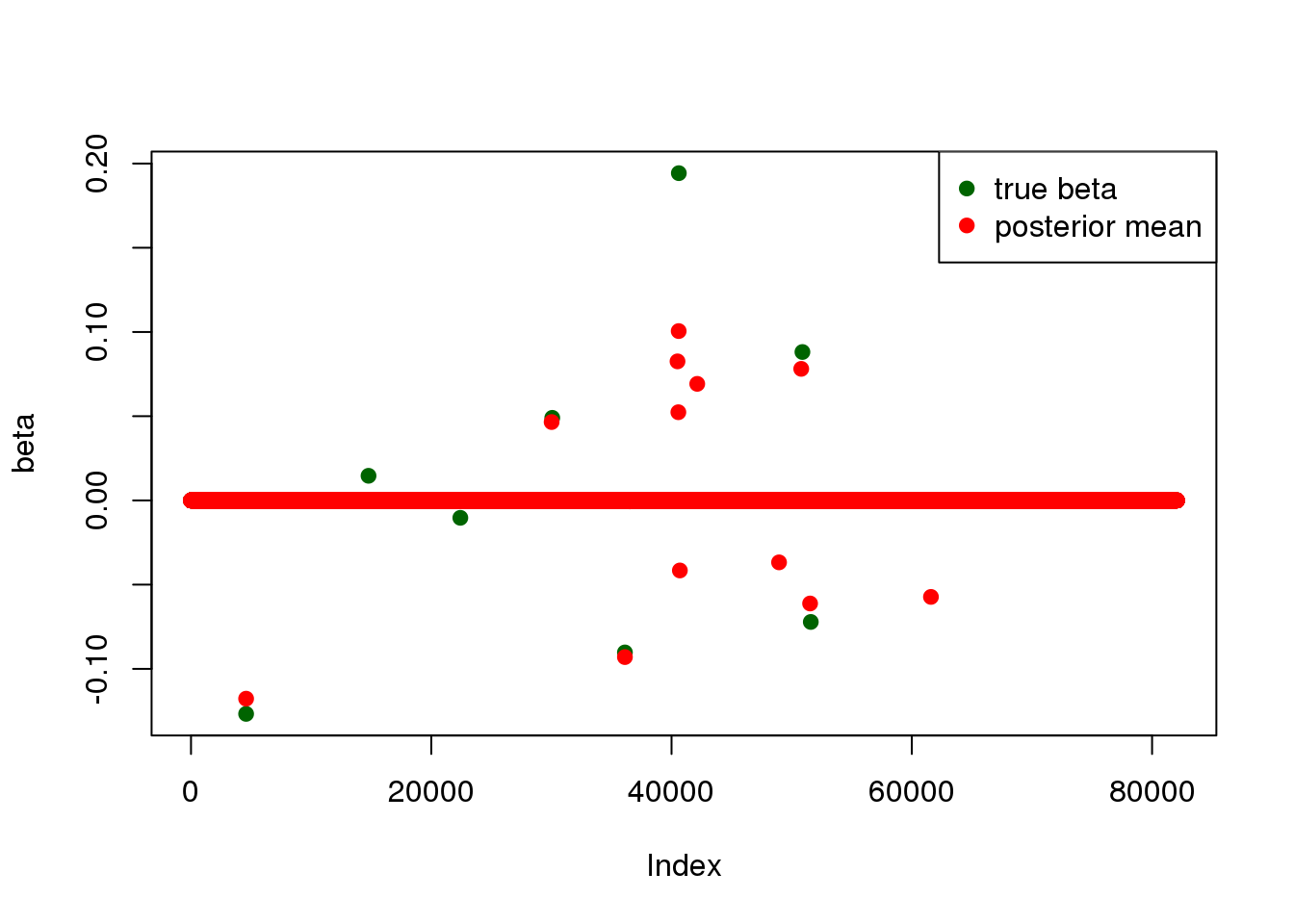
Simulation 4
True parameters:
load(paste0(simdatadir, "mr.ash2_20200503-4-pheno.Rd"))
readLines(paste0(simdatadir, "param-20200503-4.R"))
[1] "pve.expr <- 0.005" "pve.snp <- 0.01" "pi_beta <- 0.05"
[4] "pi_theta <- 1e-4" "tau <- 1" MR.ASH results (start from gene):
load(paste0(outputdir, "20200527-4-mr.ash2s.expr-res.Rd"))
g.fit <- mr.ash2s.fit$fit1
s.fit <-  mr.ash2s.fit$fit2
summary_mr.ash2(g.fit, s.fit, phenores)
gene expression effect:
pi1 = 0.03483871
pve = 0.09146919 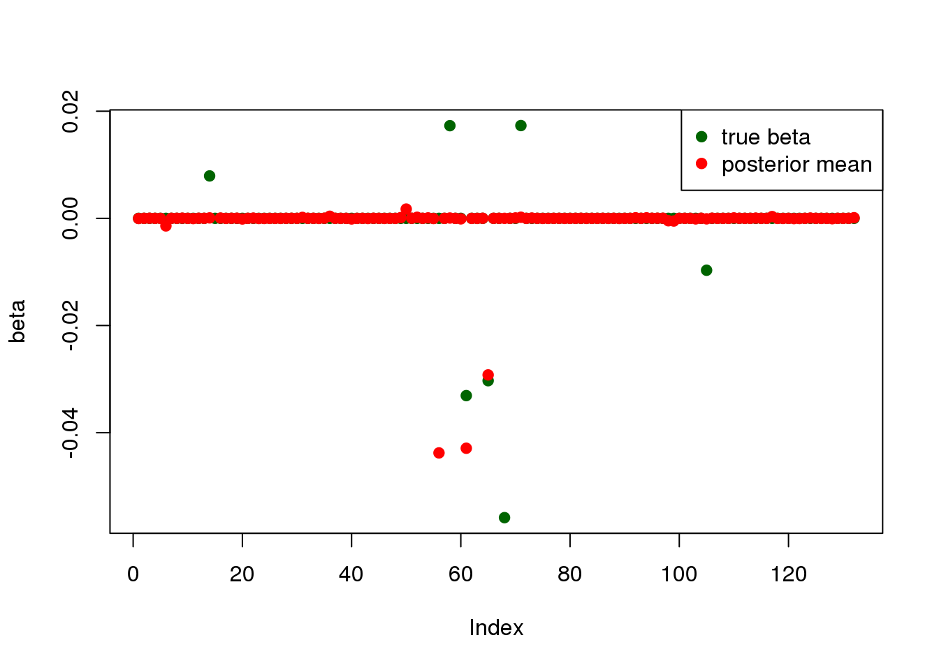

false positive rate:  0.5
false negative rate:  0.7142857
snp effect:
pi1 =  4.177662e-05
pve = 0.0699035 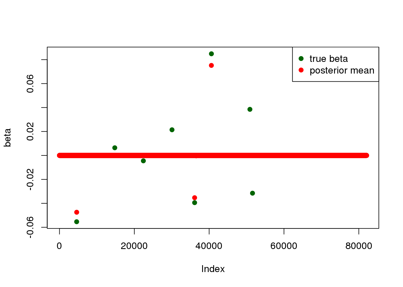
MR.ASH results (start from SNP):
load(paste0(outputdir, "20200527-4-mr.ash2s.snp-res.Rd"))
g.fit <- mr.ash2s.fit$fit2
s.fit <-  mr.ash2s.fit$fit1
summary_mr.ash2(g.fit, s.fit, phenores)
gene expression effect:
pi1 = 0.02582045
pve = 0.06943356 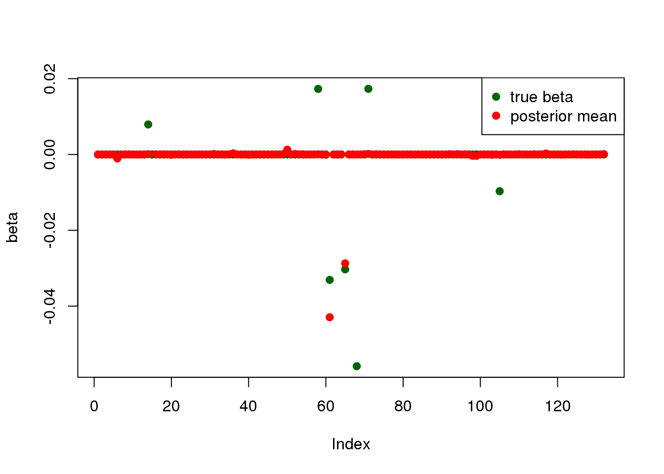
false positive rate:  0.3333333
false negative rate:  0.7142857
snp effect:
pi1 =  5.635395e-05
pve = 0.09201309 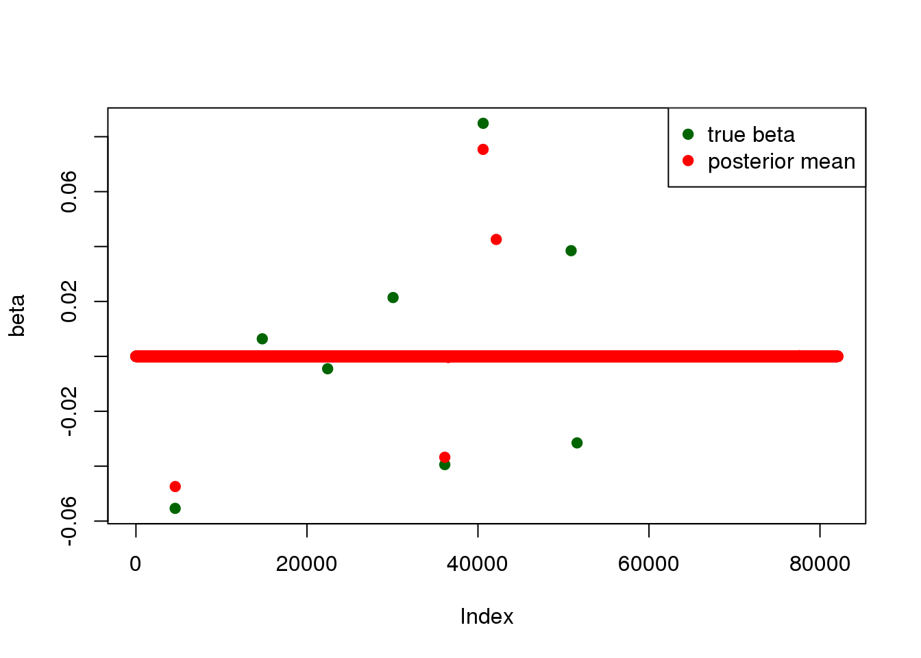
sessionInfo()R version 3.5.1 (2018-07-02)
Platform: x86_64-pc-linux-gnu (64-bit)
Running under: Scientific Linux 7.4 (Nitrogen)
Matrix products: default
BLAS/LAPACK: /software/openblas-0.2.19-el7-x86_64/lib/libopenblas_haswellp-r0.2.19.so
locale:
[1] LC_CTYPE=en_US.UTF-8 LC_NUMERIC=C
[3] LC_TIME=en_US.UTF-8 LC_COLLATE=en_US.UTF-8
[5] LC_MONETARY=en_US.UTF-8 LC_MESSAGES=en_US.UTF-8
[7] LC_PAPER=en_US.UTF-8 LC_NAME=C
[9] LC_ADDRESS=C LC_TELEPHONE=C
[11] LC_MEASUREMENT=en_US.UTF-8 LC_IDENTIFICATION=C
attached base packages:
[1] stats graphics grDevices utils datasets methods base
other attached packages:
[1] mr.ash.alpha_0.1-7
loaded via a namespace (and not attached):
[1] workflowr_1.6.0 Rcpp_1.0.4.6 lattice_0.20-38 digest_0.6.18
[5] later_0.7.5 rprojroot_1.3-2 grid_3.5.1 R6_2.3.0
[9] backports_1.1.2 git2r_0.26.1 magrittr_1.5 evaluate_0.12
[13] highr_0.7 stringi_1.3.1 fs_1.3.1 promises_1.0.1
[17] Matrix_1.2-15 rmarkdown_1.10 tools_3.5.1 stringr_1.4.0
[21] glue_1.3.0 httpuv_1.4.5 yaml_2.2.0 compiler_3.5.1
[25] htmltools_0.3.6 knitr_1.20