Summarize twas: chr17 to 22
2020-09-03
Last updated: 2020-09-03
Checks: 6 1
Knit directory: causal-TWAS/
This reproducible R Markdown analysis was created with workflowr (version 1.6.2). The Checks tab describes the reproducibility checks that were applied when the results were created. The Past versions tab lists the development history.
The R Markdown file has unstaged changes. To know which version of the R Markdown file created these results, you’ll want to first commit it to the Git repo. If you’re still working on the analysis, you can ignore this warning. When you’re finished, you can run wflow_publish to commit the R Markdown file and build the HTML.
Great job! The global environment was empty. Objects defined in the global environment can affect the analysis in your R Markdown file in unknown ways. For reproduciblity it’s best to always run the code in an empty environment.
The command set.seed(20191103) was run prior to running the code in the R Markdown file. Setting a seed ensures that any results that rely on randomness, e.g. subsampling or permutations, are reproducible.
Great job! Recording the operating system, R version, and package versions is critical for reproducibility.
Nice! There were no cached chunks for this analysis, so you can be confident that you successfully produced the results during this run.
Great job! Using relative paths to the files within your workflowr project makes it easier to run your code on other machines.
Great! You are using Git for version control. Tracking code development and connecting the code version to the results is critical for reproducibility.
The results in this page were generated with repository version 193a8df. See the Past versions tab to see a history of the changes made to the R Markdown and HTML files.
Note that you need to be careful to ensure that all relevant files for the analysis have been committed to Git prior to generating the results (you can use wflow_publish or wflow_git_commit). workflowr only checks the R Markdown file, but you know if there are other scripts or data files that it depends on. Below is the status of the Git repository when the results were generated:
Ignored files:
    Ignored:    .Rhistory
    Ignored:    .Rproj.user/
    Ignored:    code/workflow/.ipynb_checkpoints/
    Ignored:    data/

Unstaged changes:
    Modified:   analysis/simulation-multi-ukbchr17to22-gtex.adipose_susieprior.Rmd
    Modified:   analysis/simulation-susieI-ukbchr17to22-gtex.adipose.Rmd
    Modified:   code/run_test_susie.R
    Modified:   code/run_test_susieI.R
    Modified:   code/workflow/workflow-ashtest4.ipynb
    Modified:   code/workflow/workflow-susieI-20200813.ipynb
Note that any generated files, e.g. HTML, png, CSS, etc., are not included in this status report because it is ok for generated content to have uncommitted changes.
These are the previous versions of the repository in which changes were made to the R Markdown (analysis/simulation-multi-ukbchr17to22-gtex.adipose_susieprior.Rmd) and HTML (docs/simulation-multi-ukbchr17to22-gtex.adipose_susieprior.html) files. If you’ve configured a remote Git repository (see ?wflow_git_remote), click on the hyperlinks in the table below to view the files as they were in that past version.
| File | Version | Author | Date | Message |
|---|---|---|---|---|
| Rmd | 193a8df | simingz | 2020-09-01 | increase gene pve |
| html | 193a8df | simingz | 2020-09-01 | increase gene pve |
| Rmd | 86681eb | simingz | 2020-08-28 | susieI all regions |
| html | 86681eb | simingz | 2020-08-28 | susieI all regions |
`
Run susie with different priors and see how much prior affects results.
Data: ukb chr 17 to chr 22 combined. SNPs are downsampled to 1/10, eQTLs defined by FUSION-TWAS (Adipose/GTEx) lasso effect size > 0 were kept, p= 86k, n = 20k.
library(mr.ash.alpha)
library(data.table)
suppressMessages({library(plotly)})
library(tidyr)
library(plyr)
library(stringr)
library(kableExtra)
source("analysis/summarize_twas_plots.R")
Setting 1
PIP calibration: filter regions
simdatadir <- "~/causalTWAS/simulations/simulation_ashtest_20200721/"
outputdir <- "~/causalTWAS/simulations/simulation_ashtest_20200721/"
susiedir <- "~/causalTWAS/simulations/simulation_susietest_20200721/20200721-1-fixprior_rpip0.5/"
We run 100 simulations and run susie using different priors and L= 1. We only apply susie for regions with mr.ash2 regional PIP > 0.5.
Truth
- The true parameters we used to simulate data:
par <- read.table(paste0(susiedir, "20200721-1-fixedprior_1.txt"), header = T)
t(par[,2, drop = F])
gene.pi1 gene.pve snp.pi1 snp.pve
truth 0.05021174 0.008497975 0.002498094 0.05003487Using uniform prior:
pipfs <- Sys.glob(paste0(susiedir,"20200721-1-*.fixedprior1.L1.susieres.expr.txt"))
res <- do.call(rbind, lapply(pipfs, read.table, header = T))
cp_plot(res$pip.null, res$ifcausal, main = "SUSIE.uniform PIP")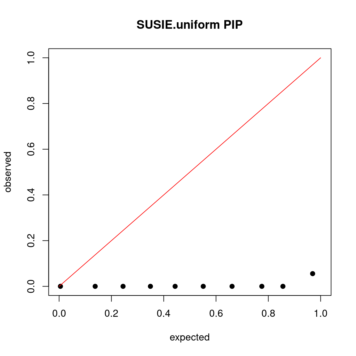
Use overestimated prior
- The prior used is:
par <- read.table(paste0(susiedir, "20200721-1-fixedprior_1.txt"), header = T)
t(par[c(1,3),1, drop = F])
gene.pi1 snp.pi1
estimated 0.131184 0.002274899- susie results:
par(mfrow=c(1,2))
cp_plot(res$pip, res$ifcausal, main = "SUSIE.weighted PIP")
cp_plot(res$pip.w0, res$ifcausal, main = "SUSIE.weighted-w-null PIP")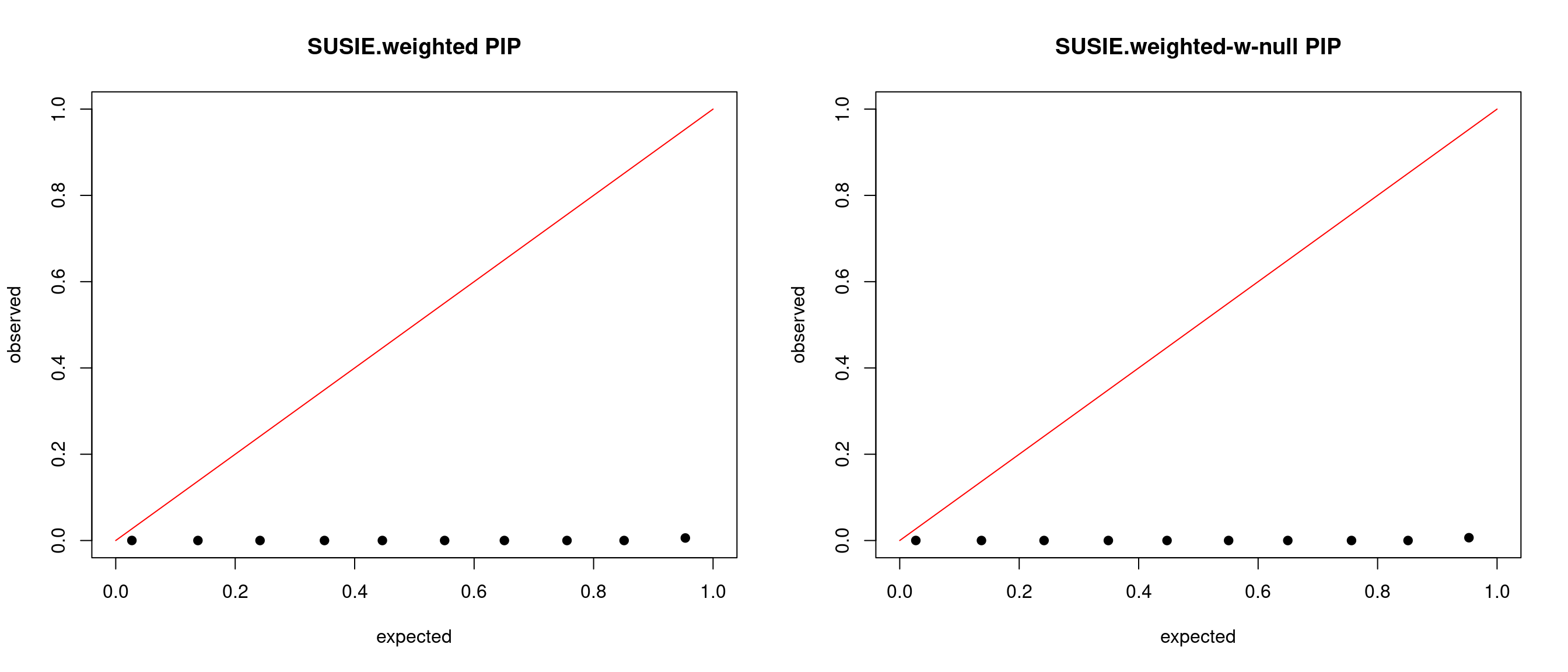
Use priors close to truth
- The prior used is:
par <- read.table(paste0(susiedir, "20200721-1-fixedprior_2.txt"), header = T)
t(par[c(1,3),1, drop = F])
gene.pi1 snp.pi1
estimated 0.05118395 0.002274899pipfs <- Sys.glob(paste0(susiedir,"20200721-1-*.fixedprior2.L1.susieres.expr.txt"))
res <- do.call(rbind, lapply(pipfs, read.table, header = T))
par(mfrow=c(1,2))
cp_plot(res$pip, res$ifcausal, main = "SUSIE.weighted PIP")
cp_plot(res$pip.w0, res$ifcausal, main = "SUSIE.weighted-w-null PIP")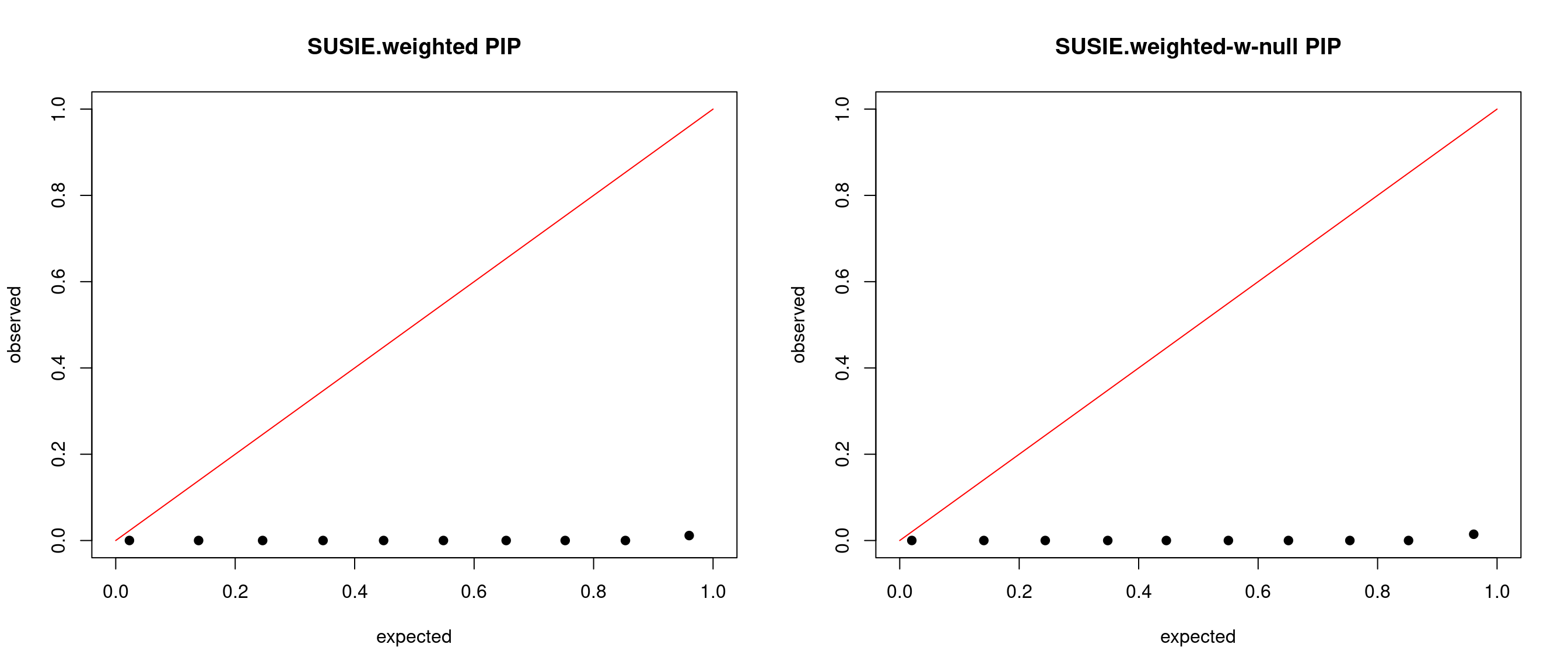
Use under estimated priors
- The prior used is:
par <- read.table(paste0(susiedir, "20200721-1-fixedprior_3.txt"), header = T)
t(par[c(1,3),1, drop = F])
gene.pi1 snp.pi1
estimated 0.01118395 0.002274899- susie results:
pipfs <- Sys.glob(paste0(susiedir,"20200721-1-*.fixedprior3.L1.susieres.expr.txt"))
res <- do.call(rbind, lapply(pipfs, read.table, header = T))
par(mfrow=c(1,2))
cp_plot(res$pip, res$ifcausal, main = "SUSIE.weighted PIP")
cp_plot(res$pip.w0, res$ifcausal, main = "SUSIE.weighted-w-null PIP")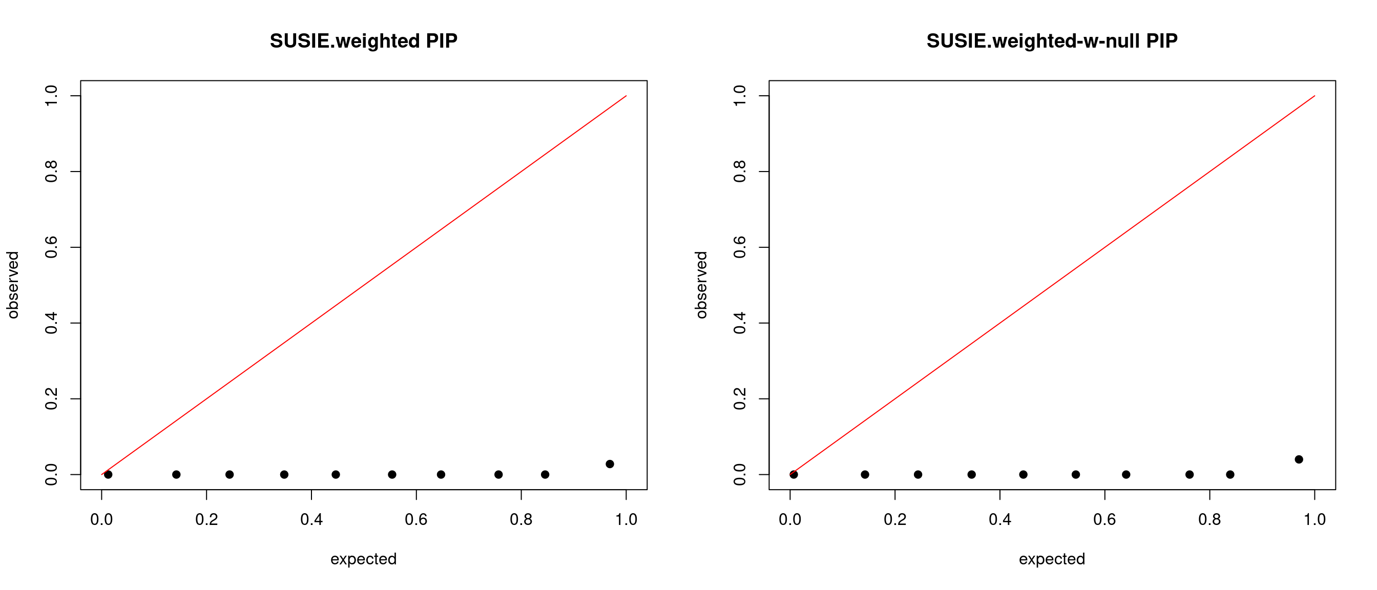
PIP calibration: all regions
susiedir <- "~/causalTWAS/simulations/simulation_susietest_20200721/"We run 50 simulations and run susie using different priors and L= 1. We apply susie for all regions.
Truth
- The true parameters we used to simulate data:
par <- read.table(paste0(susiedir, "20200721-1-fixedprior_1.txt"), header = T)
t(par[,2, drop = F])
gene.pi1 gene.pve snp.pi1 snp.pve
truth 0.05021174 0.008497975 0.002498094 0.05003487Using uniform prior:
pipfs <- Sys.glob(paste0(susiedir,"20200721-1-*.fixedprior1.L1.susieres.expr.txt"))
res <- do.call(rbind, lapply(pipfs, read.table, header = T))

cp_plot(res$pip.null, res$ifcausal, main = "SUSIE.uniform PIP")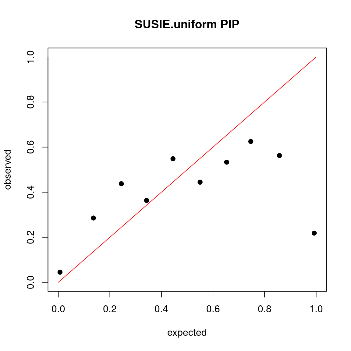
Use overestimated prior
- The prior used is:
par <- read.table(paste0(susiedir, "20200721-1-fixedprior_1.txt"), header = T)
t(par[c(1,3),1, drop = F])
gene.pi1 snp.pi1
estimated 0.131184 0.002274899- susie results:
par(mfrow=c(1,2))
cp_plot(res$pip, res$ifcausal, main = "SUSIE.weighted PIP")
cp_plot(res$pip.w0, res$ifcausal, main = "SUSIE.weighted-w-null PIP")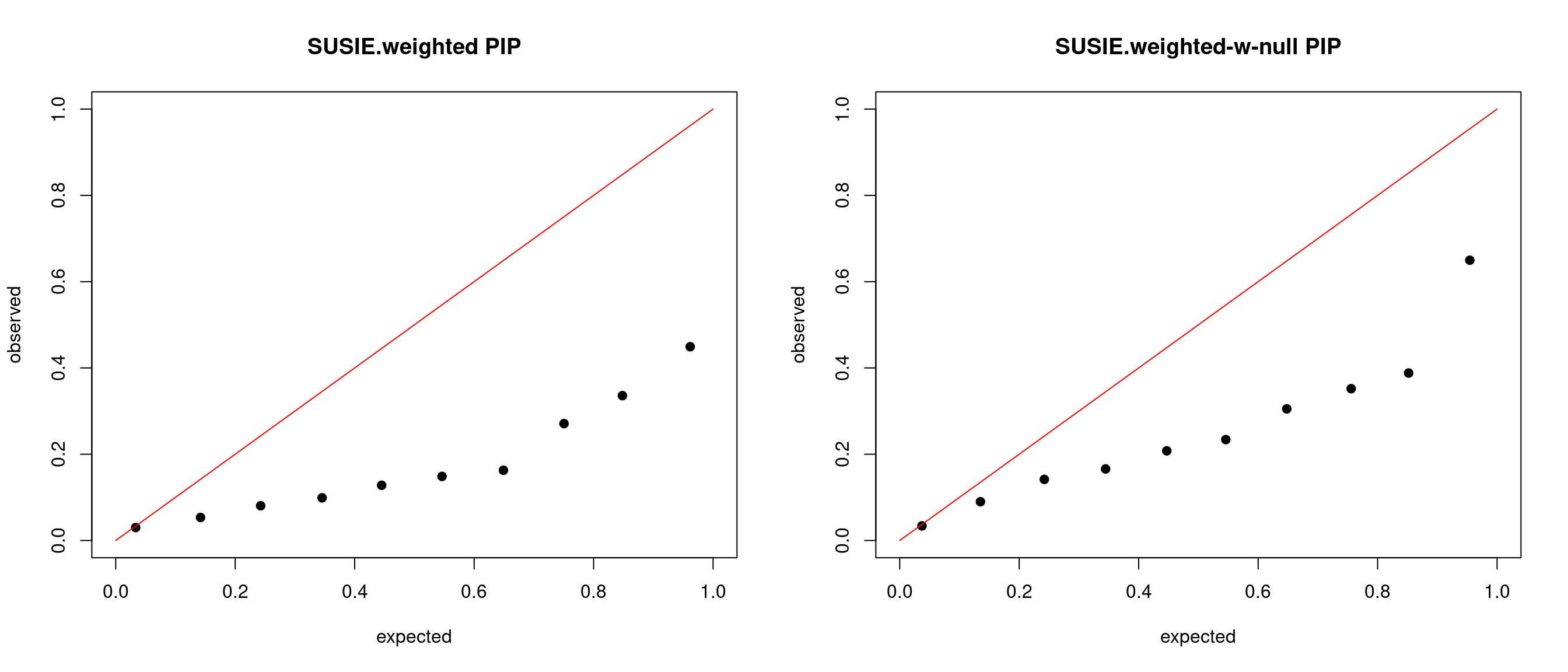
Use priors close to truth
- The prior used is:
par <- read.table(paste0(susiedir, "20200721-1-fixedprior_2.txt"), header = T)
t(par[c(1,3),1, drop = F])
gene.pi1 snp.pi1
estimated 0.05118395 0.002274899pipfs <- Sys.glob(paste0(susiedir,"20200721-1-*.fixedprior2.L1.susieres.expr.txt"))
res <- do.call(rbind, lapply(pipfs, read.table, header = T))
par(mfrow=c(1,2))
cp_plot(res$pip, res$ifcausal, main = "SUSIE.weighted PIP")
cp_plot(res$pip.w0, res$ifcausal, main = "SUSIE.weighted-w-null PIP")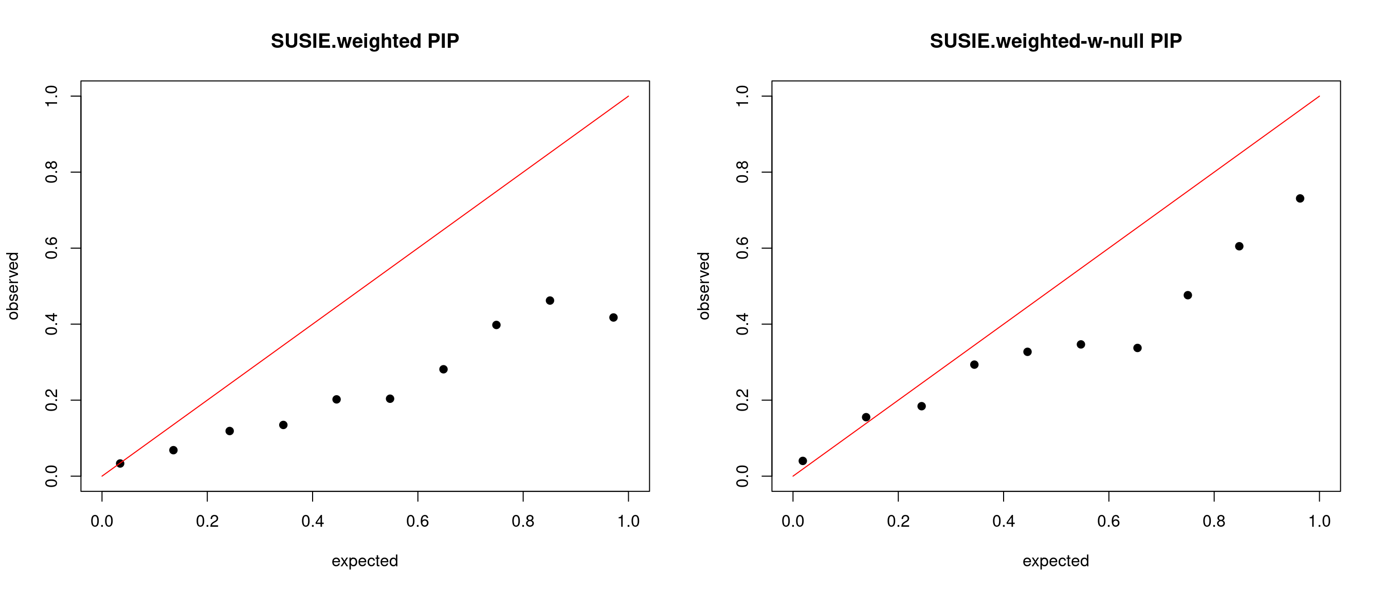
Use under estimated priors
- The prior used is:
par <- read.table(paste0(susiedir, "20200721-1-fixedprior_3.txt"), header = T)
t(par[c(1,3),1, drop = F])
gene.pi1 snp.pi1
estimated 0.01118395 0.002274899- susie results:
pipfs <- Sys.glob(paste0(susiedir,"20200721-1-*.fixedprior3.L1.susieres.expr.txt"))
res <- do.call(rbind, lapply(pipfs, read.table, header = T))

par(mfrow=c(1,2))
cp_plot(res$pip, res$ifcausal, main = "SUSIE.weighted PIP")
cp_plot(res$pip.w0, res$ifcausal, main = "SUSIE.weighted-w-null PIP")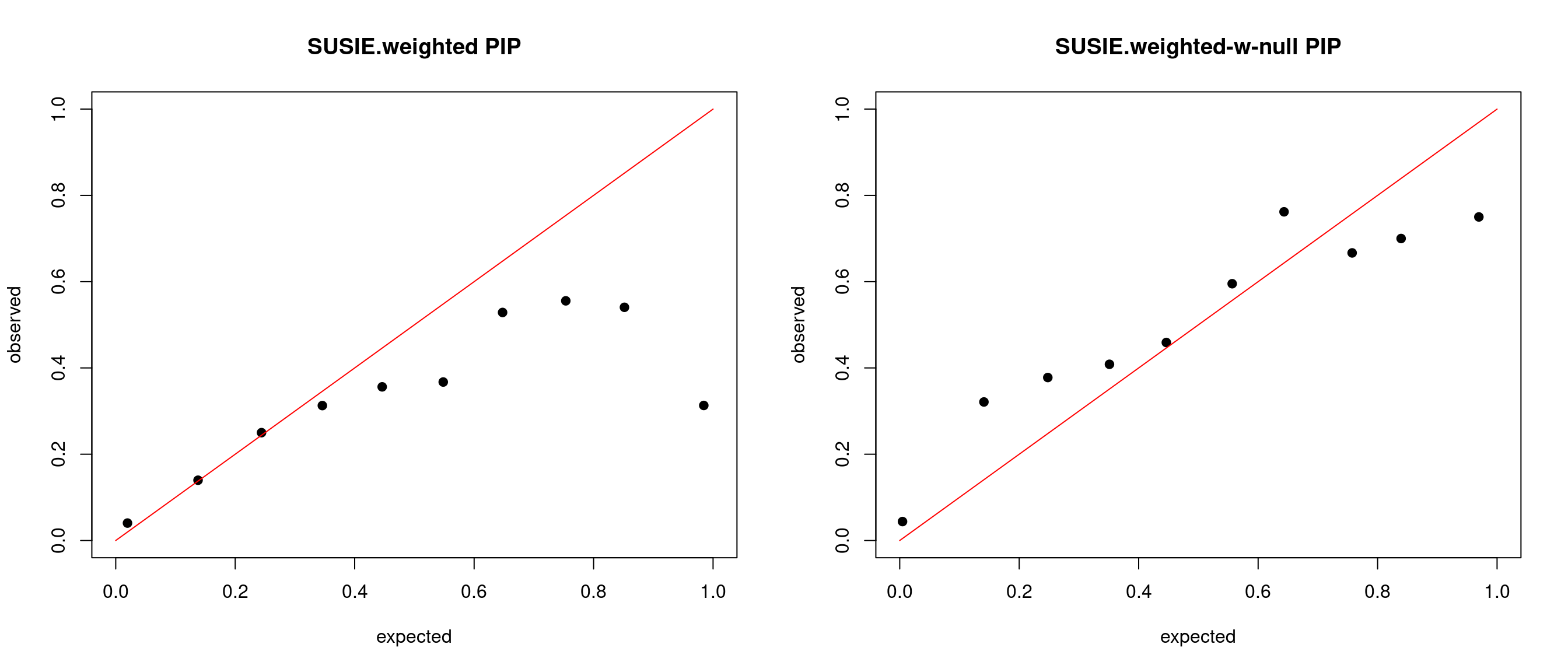
Setting 2
PIP calibration: filter regions
susiedir <- "~/causalTWAS/simulations/simulation_susietest_20200721/20200721-3-fixprior_causal/"We run 100 simulations and run susie using different priors and L= 1. We only apply susie for regions with at least one causal signal.
Truth
- The true parameters we used to simulate data:
par <- read.table(paste0(susiedir, "20200721-3-fixedprior_1.txt"), header = T)
t(par[,2, drop = F])
gene.pi1 gene.pve snp.pi1 snp.pve
truth 0.0199637 0.007322058 0.002498094 0.05257447Using uniform prior:
pipfs <- Sys.glob(paste0(susiedir,"20200721-3-*.fixedprior1.L1.susieres.expr.txt"))
res <- do.call(rbind, lapply(pipfs, read.table, header = T))
cp_plot(res$pip.null, res$ifcausal, main = "SUSIE.uniform PIP")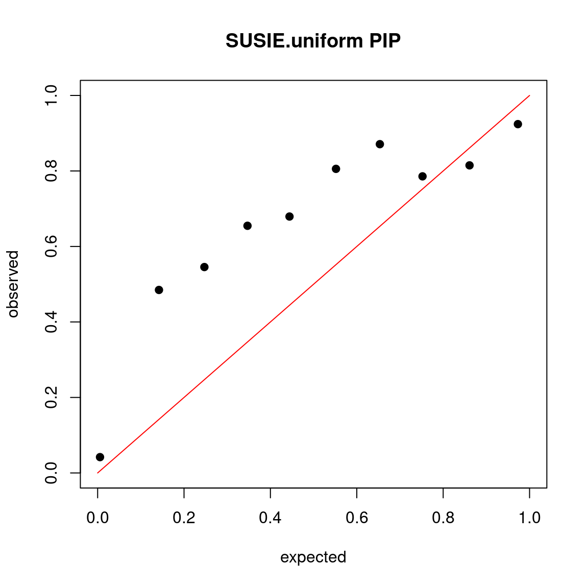
Use overestimated prior
- The prior used is:
par <- read.table(paste0(susiedir, "20200721-3-fixedprior_1.txt"), header = T)
t(par[c(1,3),1, drop = F])
gene.pi1 snp.pi1
estimated 0.1054679 0.0030996- susie results:
par(mfrow=c(1,2))
cp_plot(res$pip, res$ifcausal, main = "SUSIE.weighted PIP")
cp_plot(res$pip.w0, res$ifcausal, main = "SUSIE.weighted-w-null PIP")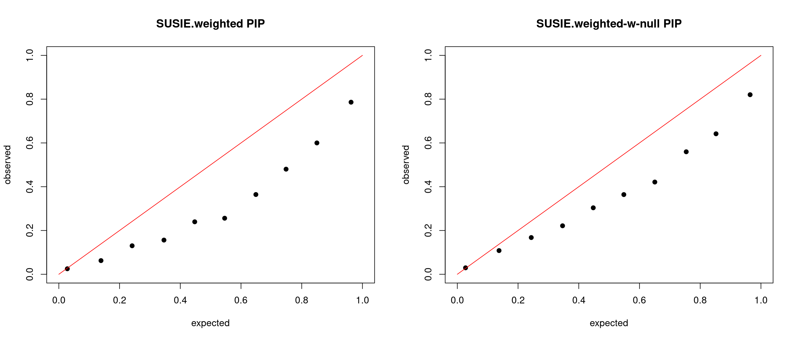
Use priors close to truth
- The prior used is:
par <- read.table(paste0(susiedir, "20200721-3-fixedprior_2.txt"), header = T)
t(par[c(1,3),1, drop = F])
gene.pi1 snp.pi1
estimated 0.02 0.0030996- susie results:
pipfs <- Sys.glob(paste0(susiedir,"20200721-3-*.fixedprior2.L1.susieres.expr.txt"))
res <- do.call(rbind, lapply(pipfs, read.table, header = T))
par(mfrow=c(1,2))
cp_plot(res$pip, res$ifcausal, main = "SUSIE.weighted PIP")
cp_plot(res$pip.w0, res$ifcausal, main = "SUSIE.weighted-w-null PIP")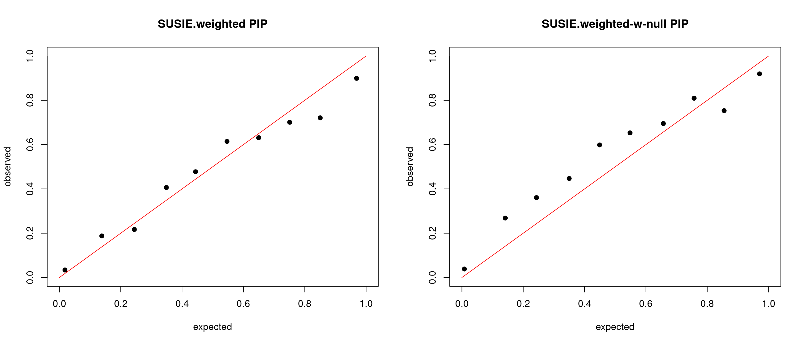
Use under estimated priors
- The prior used is:
par <- read.table(paste0(susiedir, "20200721-3-fixedprior_3.txt"), header = T)
t(par[c(1,3),1, drop = F])
gene.pi1 snp.pi1
estimated 0.01 0.0030996- susie results:
pipfs <- Sys.glob(paste0(susiedir,"20200721-3-*.fixedprior3.L1.susieres.expr.txt"))
res <- do.call(rbind, lapply(pipfs, read.table, header = T))
par(mfrow=c(1,2))
cp_plot(res$pip, res$ifcausal, main = "SUSIE.weighted PIP")
cp_plot(res$pip.w0, res$ifcausal, main = "SUSIE.weighted-w-null PIP")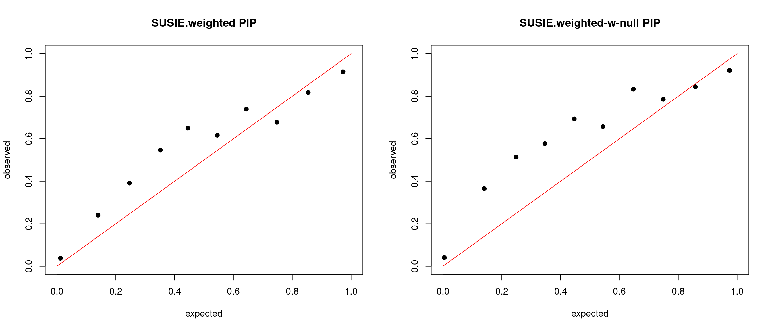
PIP calibration: all regions
susiedir <- "~/causalTWAS/simulations/simulation_susietest_20200721/"We run 100 simulations and run susie using different priors and L= 1. We only apply susie for all regions.
Truth
- The true parameters we used to simulate data:
par <- read.table(paste0(susiedir, "20200721-3-fixedprior_1.txt"), header = T)
t(par[,2, drop = F])
gene.pi1 gene.pve snp.pi1 snp.pve
truth 0.0199637 0.007322058 0.002498094 0.05257447Using uniform prior:
pipfs <- Sys.glob(paste0(susiedir,"20200721-3-*.fixedprior1.L1.susieres.expr.txt"))
res <- do.call(rbind, lapply(pipfs, read.table, header = T))

cp_plot(res$pip.null, res$ifcausal, main = "SUSIE.uniform PIP")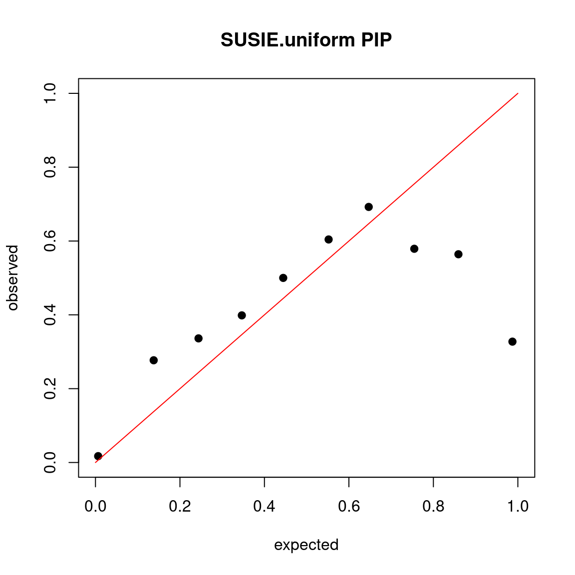
Use overestimated prior
- The prior used is:
par <- read.table(paste0(susiedir, "20200721-3-fixedprior_1.txt"), header = T)
t(par[c(1,3),1, drop = F])
gene.pi1 snp.pi1
estimated 0.1054679 0.0030996- susie results:
par(mfrow=c(1,2))
cp_plot(res$pip, res$ifcausal, main = "SUSIE.weighted PIP")
cp_plot(res$pip.w0, res$ifcausal, main = "SUSIE.weighted-w-null PIP")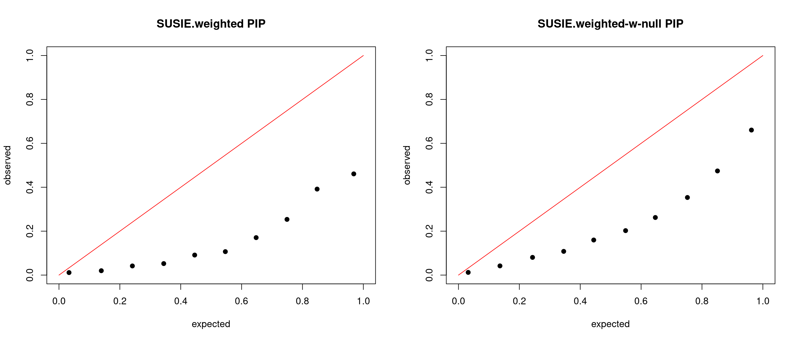
Use priors close to truth
- The prior used is:
par <- read.table(paste0(susiedir, "20200721-3-fixedprior_2.txt"), header = T)
t(par[c(1,3),1, drop = F])
gene.pi1 snp.pi1
estimated 0.02 0.0030996- susie results:
pipfs <- Sys.glob(paste0(susiedir,"20200721-3-*.fixedprior2.L1.susieres.expr.txt"))
res <- do.call(rbind, lapply(pipfs, read.table, header = T))

par(mfrow=c(1,2))
cp_plot(res$pip, res$ifcausal, main = "SUSIE.weighted PIP")
cp_plot(res$pip.w0, res$ifcausal, main = "SUSIE.weighted-w-null PIP")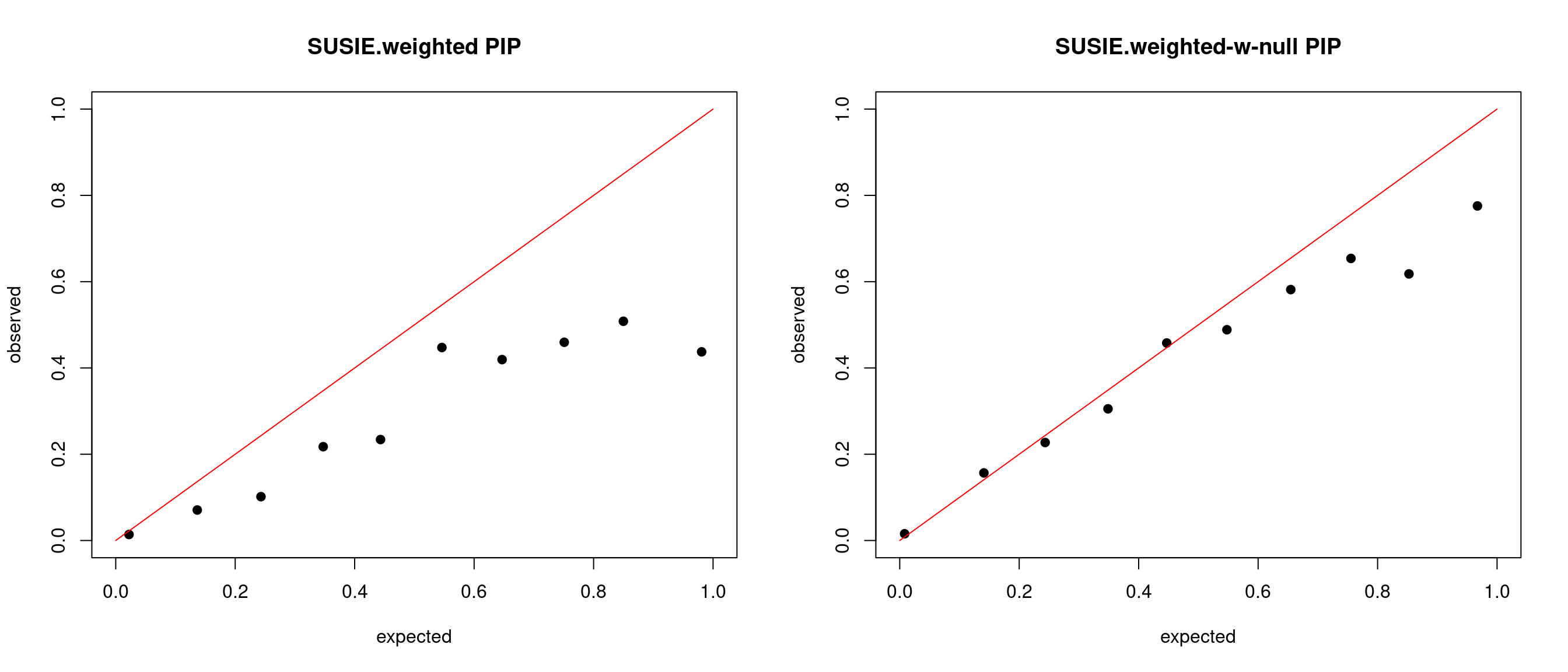
Use under estimated priors
- The prior used is:
par <- read.table(paste0(susiedir, "20200721-3-fixedprior_3.txt"), header = T)
t(par[c(1,3),1, drop = F])
gene.pi1 snp.pi1
estimated 0.01 0.0030996- susie results:
pipfs <- Sys.glob(paste0(susiedir,"20200721-3-*.fixedprior3.L1.susieres.expr.txt"))
res <- do.call(rbind, lapply(pipfs, read.table, header = T))

par(mfrow=c(1,2))
cp_plot(res$pip, res$ifcausal, main = "SUSIE.weighted PIP")
cp_plot(res$pip.w0, res$ifcausal, main = "SUSIE.weighted-w-null PIP")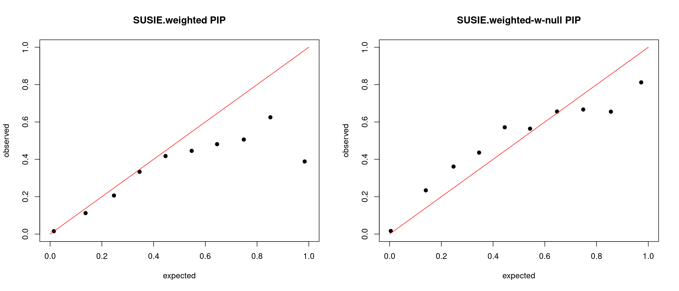
sessionInfo()R version 3.5.1 (2018-07-02)
Platform: x86_64-pc-linux-gnu (64-bit)
Running under: Scientific Linux 7.4 (Nitrogen)
Matrix products: default
BLAS/LAPACK: /software/openblas-0.2.19-el7-x86_64/lib/libopenblas_haswellp-r0.2.19.so
locale:
[1] LC_CTYPE=en_US.UTF-8 LC_NUMERIC=C
[3] LC_TIME=en_US.UTF-8 LC_COLLATE=en_US.UTF-8
[5] LC_MONETARY=en_US.UTF-8 LC_MESSAGES=en_US.UTF-8
[7] LC_PAPER=en_US.UTF-8 LC_NAME=C
[9] LC_ADDRESS=C LC_TELEPHONE=C
[11] LC_MEASUREMENT=en_US.UTF-8 LC_IDENTIFICATION=C
attached base packages:
[1] stats graphics grDevices utils datasets methods base
other attached packages:
[1] kableExtra_1.2.1 stringr_1.4.0 plyr_1.8.6
[4] tidyr_0.8.3 plotly_4.9.2.9000 ggplot2_3.3.1
[7] data.table_1.12.7 mr.ash.alpha_0.1-34
loaded via a namespace (and not attached):
[1] Rcpp_1.0.4.6 compiler_3.5.1 pillar_1.4.4
[4] later_0.7.5 git2r_0.26.1 workflowr_1.6.2
[7] tools_3.5.1 digest_0.6.25 viridisLite_0.3.0
[10] jsonlite_1.6.1 evaluate_0.12 tibble_3.0.1
[13] lifecycle_0.2.0 gtable_0.2.0 lattice_0.20-38
[16] pkgconfig_2.0.2 rlang_0.4.6 Matrix_1.2-15
[19] rstudioapi_0.11 yaml_2.2.0 xml2_1.2.0
[22] httr_1.4.1 withr_2.1.2 dplyr_1.0.0
[25] knitr_1.20 htmlwidgets_1.3 generics_0.0.2
[28] fs_1.3.1 vctrs_0.3.1 webshot_0.5.1
[31] tidyselect_1.1.0 rprojroot_1.3-2 grid_3.5.1
[34] glue_1.4.1 R6_2.3.0 rmarkdown_1.10
[37] purrr_0.3.4 magrittr_1.5 whisker_0.3-2
[40] backports_1.1.2 scales_1.0.0 promises_1.0.1
[43] htmltools_0.3.6 ellipsis_0.3.1 rvest_0.3.2
[46] colorspace_1.3-2 httpuv_1.4.5 stringi_1.3.1
[49] lazyeval_0.2.1 munsell_0.5.0 crayon_1.3.4