Paper figures (Simulation)

Parameter estimation

Parameter vs. true value
Comparison of PVE.gene vs. MESC estimates.

PIP calibration

PIP plot under different settings.
Comparison with other methods

Examples

FP example 1
FP example 2
TP example

Last updated: 2021-07-31

Checks: 5 2

Knit directory: causal-TWAS/

This reproducible R Markdown analysis was created with workflowr (version 1.6.2). The Checks tab describes the reproducibility checks that were applied when the results were created. The Past versions tab lists the development history.

R Markdown file: uncommitted changes

The R Markdown is untracked by Git. To know which version of the R Markdown file created these results, you'll want to first commit it to the Git repo. If you're still working on the analysis, you can ignore this warning. When you're finished, you can run wflow_publish to commit the R Markdown file and build the HTML.

Environment: empty

Great job! The global environment was empty. Objects defined in the global environment can affect the analysis in your R Markdown file in unknown ways. For reproduciblity it's best to always run the code in an empty environment.

Seed: set.seed(20191103)

The command set.seed(20191103) was run prior to running the code in the R Markdown file. Setting a seed ensures that any results that rely on randomness, e.g. subsampling or permutations, are reproducible.

Session information: recorded

Great job! Recording the operating system, R version, and package versions is critical for reproducibility.

Cache: none

Nice! There were no cached chunks for this analysis, so you can be confident that you successfully produced the results during this run.

File paths: absolute

Using absolute paths to the files within your workflowr project makes it difficult for you and others to run your code on a different machine. Change the absolute path(s) below to the suggested relative path(s) to make your code more reproducible.

absolute	relative
~/causalTWAS/causal-TWAS/analysis/summarize_basic_plots.R	analysis/summarize_basic_plots.R
~/causalTWAS/causal-TWAS/analysis/summarize_ctwas_plots.R	analysis/summarize_ctwas_plots.R
~/causalTWAS/causal-TWAS/analysis/ld.R	analysis/ld.R

Repository version: 6dee9b0

Great! You are using Git for version control. Tracking code development and connecting the code version to the results is critical for reproducibility.

The results in this page were generated with repository version 6dee9b0. See the Past versions tab to see a history of the changes made to the R Markdown and HTML files.

Note that you need to be careful to ensure that all relevant files for the analysis have been committed to Git prior to generating the results (you can use wflow_publish or wflow_git_commit). workflowr only checks the R Markdown file, but you know if there are other scripts or data files that it depends on. Below is the status of the Git repository when the results were generated:


Ignored files:
    Ignored:    .Rhistory
    Ignored:    .Rproj.user/
    Ignored:    .ipynb_checkpoints/
    Ignored:    analysis/.ipynb_checkpoints/
    Ignored:    code/.ipynb_checkpoints/
    Ignored:    code/before_package/.ipynb_checkpoints/
    Ignored:    code/workflow/.ipynb_checkpoints/
    Ignored:    data/

Untracked files:
    Untracked:  analysis/Paper_figures_simulation.Rmd
    Untracked:  analysis/ld.R

Unstaged changes:
    Modified:   analysis/index.Rmd
    Modified:   analysis/simulation-ctwas-ukbWG-gtex.adipose_visual.Rmd
    Modified:   analysis/summarize_basic_plots.R
    Modified:   analysis/summarize_ctwas_plots.R

Note that any generated files, e.g. HTML, png, CSS, etc., are not included in this status report because it is ok for generated content to have uncommitted changes.

There are no past versions. Publish this analysis with wflow_publish() to start tracking its development.

library(ctwas)
library(data.table)
source("~/causalTWAS/causal-TWAS/analysis/summarize_basic_plots.R")


********************************************************

Note: As of version 1.0.0, cowplot does not change the

  default ggplot2 theme anymore. To recover the previous

  behavior, execute:
  theme_set(theme_cowplot())

********************************************************


Attaching package: 'ggpubr'

The following object is masked from 'package:cowplot':

    get_legend

source("~/causalTWAS/causal-TWAS/analysis/summarize_ctwas_plots.R")
source("~/causalTWAS/causal-TWAS/analysis/ld.R")

outputdir = "/home/simingz/causalTWAS/simulations/simulation_ctwas_rss_20210416/"
comparedir = "/home/simingz/causalTWAS/simulations/simulation_ctwas_rss_20210416_compare/"
runtag = "ukb-s80.45-adi"
configtag = 1
pgenfn = "/home/simingz/causalTWAS/ukbiobank/ukb_pgen_s80.45/ukb-s80.45_pgenfs.txt"
exprfn = "/home/simingz/causalTWAS/simulations/simulation_ctwas_rss_20210416//ukb-s80.45-adi.expr.txt"

pgenfs <- read.table(pgenfn, header = F, stringsAsFactors = F)[,1]
pvarfs <- sapply(pgenfs, prep_pvar, outputdir = outputdir)
pgens <- lapply(1:length(pgenfs), function(x) prep_pgen(pgenf = pgenfs[x],pvarf = pvarfs[x]))
exprfs <- read.table(exprfn, header = F, stringsAsFactors = F)[,1]
exprvarfs <- sapply(exprfs, prep_exprvar)

n <- pgenlibr::GetRawSampleCt(pgens[[1]])
p <- sum(unlist(lapply(pgens, pgenlibr::GetVariantCt))) # number of SNPs
J <- 8021 # number of genes

colorsall <- c("#7fc97f", "#beaed4", "#fdc086")

Parameter estimation

Parameter vs. true value

Each plot show one parameter: pi.gene, pi.gene/pi.SNP (enrichment), effectsize.gene, PVE.gene, horizontal bar shows true values, and multiple dots, each show one setting.

plot_single <- function(mtxlist, truecol, estcol, ...){
  truth <- do.call(rbind, lapply(1:length(mtxlist), function(x) cbind(x, mean(mtxlist[[x]][, truecol]))))
  est <- do.call(rbind, lapply(1:length(mtxlist), function(x) cbind(x, mtxlist[[x]][, estcol])))
  
  col = est[,1]
  est[,1] <- jitter(est[,1])

  plot(est, pch = 19, xaxt = "n", xlab="" ,frame.plot=FALSE, col = colorsall[col], ...)
  axis(side=1, at=1:2, labels = c("setting 1", "setting 2"), tick = F)
  #text(x=1:length(mtxlist), 0, labels = paste0("temp",1:length(mtxlist)), xpd = T, pos =1)
  for (t in 1:nrow(truth)){
    row <- truth[t,]
    segments(row[1]-0.2, row[2] , row[1] + 0.2, row[2],
       col = colorsall[t], lty = par("lty"), lwd = 2, xpd = FALSE)
  }
  grid()
}
 

plot_par <- function(configtag, runtag, simutaglist){
  mtxlist <- list()
  for (group in 1:length(simutaglist)){
    simutags <- simutaglist[[group]]
    source(paste0(outputdir, "config", configtag, ".R"))
    phenofs <- paste0(outputdir, runtag, "_simu", simutags, "-pheno.Rd")
    susieIfs <- paste0(outputdir, runtag, "_simu", simutags, "_config", configtag, ".s2.susieIrssres.Rd")
    susieIfs2 <- paste0(outputdir, runtag, "_simu",simutags, "_config", configtag,".s2.susieIrss.txt")
    mtxlist[[group]] <- show_param(phenofs, susieIfs, susieIfs2, thin = thin)
  }
  
  # pi1 
  par(mfrow=c(1,4))
  plot_single(mtxlist, truecol = "pi1.gene_truth", estcol = "pi1.gene_est", ylab ="gene pi1", ylim = c(0,0.02), xlim = c(0.8,2.4))
  plot_single(mtxlist, truecol = "enrich_truth", estcol = "enrich_est",ylab ="gene enrichment", ylim = c(0,120), xlim = c(0.8,2.4) )
  plot_single(mtxlist, truecol = "sigma.gene_truth", estcol = "sigma.gene_est", ylab = "gene effect size", ylim = c(0.01, 0.03), xlim = c(0.8,2.4))
  plot_single(mtxlist, truecol = "PVE.gene_truth", estcol = "PVE.gene_est", ylab ="gene PVE", ylim = c(0, 0.1), xlim = c(0.8,2.4))
  
  return(mtxlist)
}

Figure (supplementary):

simutaglist = list(paste(4, 1:5, sep = "-"), paste(10, 1:5, sep="-"))
mtxlist <- plot_par(configtag, runtag, simutaglist)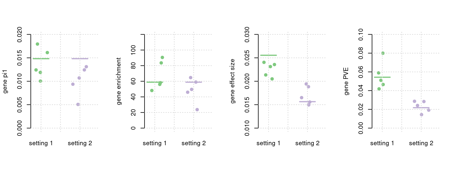

Back up figures

I have in total 10 x 2 = 20 settings to use generate the parameter figures.

Comparison of PVE.gene vs. MESC estimates.

Leave it to Kevin.

PIP calibration

PIP plot under different settings.

plot_PIP <- function(configtag, runtag,  simutags, ...){
   phenofs <- paste0(outputdir, "ukb-s80.45-adi", "_simu", simutags, "-pheno.Rd")
   susieIfs <- paste0(outputdir, runtag, "_simu",simutags, "_config", configtag,".susieIrss.txt")

   f1 <- caliPIP_plot(phenofs, susieIfs, ...) 
   return(f1)
}

simutaglist = list(paste(4, 1:5, sep = "-"), paste(10, 1:5, sep="-"))
f1 <- plot_PIP(configtag, runtag, simutaglist[[1]], main = "setting 1")
f2 <-  plot_PIP(configtag, runtag, simutaglist[[2]], main = "setting 2")
gridExtra::grid.arrange(f1, f2, ncol =2)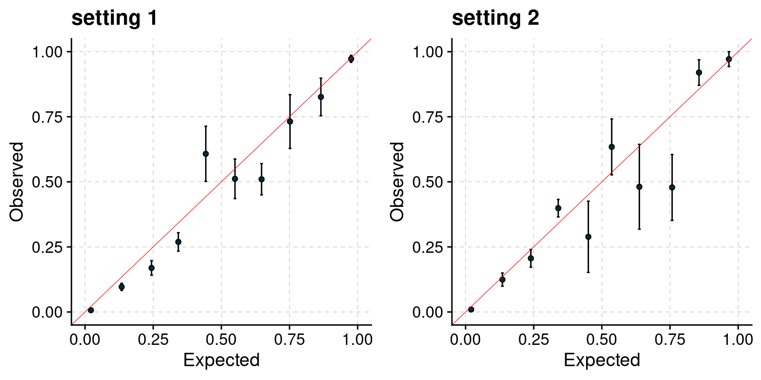

Comparison with other methods

Bar plot: each bar shows the number of genes, colored by causal status. Use a different color for each method. The method and cut off values: * ctwas: PIP 0.8 * FUSION fdr: 0.05 * FUSION bonferroni: 0.05 * COLOC PP4: 0.8 * FOCUS PIP: 0.8 * SMR FDR: 0.05 * SMR HEIDI: HEIDI p > 0.05, SMR FDR < 0.05

Multiple bar plots, different settings: high gene power and low gene power.

get_ncausal_df <- function(pfiles, cau, cut = 0.8, 
                           method = c("ctwas", "fusionfdr", "fusionbon","coloc", "focus", "smr", "smrheidi")){
  df <- NULL
  for (i in 1:length(pfiles)) {
    res <- fread(pfiles[i], header = T)
    # res <- res[complete.cases(res),]
    if (method == "ctwas"){
        res <- data.frame(res[res$type  =="gene", ])
        res$ifcausal <- ifelse(res$id %in% cau[[i]], 1, 0)
        res <- res[res$susie_pip > cut,]
    } else if (method == "fusionfdr"){
        res$FDR <- p.adjust(res$TWAS.P, method = "fdr")
        res <- res[res$FDR < cut,]
        res$ifcausal <- ifelse(res$ID %in% cau[[i]], 1, 0)
    } else if  (method == "fusionbon"){
        res$FDR <- p.adjust(res$TWAS.P, method = "bonferroni")
        res <- res[res$FDR < cut,]
        res$ifcausal <- ifelse(res$ID %in% cau[[i]], 1, 0)
    } else if  (method == "coloc"){
        res <- res[res$COLOC.PP4 > cut,]
        res$ifcausal <- ifelse(res$ID %in% cau[[i]], 1, 0)
    } else if (method == "focus"){
        res <- res[res$mol_name != "NULL",]
        res <- res[res$pip > cut, ] 
        res$ifcausal <- ifelse(res$mol_name %in% cau[[i]], 1, 0)
    } else if (method == "smr"){
        res$FDR <- p.adjust(res$p_SMR, method = "fdr")
        res <- res[res$FDR < cut,]
        res$ifcausal <- ifelse(res$probeID %in% cau[[i]], 1, 0)
    } else if (method == "smrheidi"){
        res <- res[res$p_HEIDI > 0.05,]
        res$FDR <- p.adjust(res$p_SMR, method = "fdr")
        res <- res[res$FDR < cut,]
        res$ifcausal <- ifelse(res$probeID %in% cau[[i]], 1, 0)
    } else{
      stop("no such method")
    }

    df.rt <- rbind(c(nrow(res[res$ifcausal == 0, ]), 0, i),
                   c(nrow(res[res$ifcausal == 1, ]), 1, i))
    df <- rbind(df, df.rt)
  }
  colnames(df) <- c("count", "ifcausal", "runtag")
  df <- data.frame(df)
  df$method <- method
  return(df)
}

plot_ncausal <- function(configtag, runtag,  simutags, colors, ...){
  phenofs <- paste0(outputdir, runtag, "_simu", simutags, "-pheno.Rd")
  cau <- lapply(phenofs, function(x) {load(x);get_causal_id(phenores)})
  
  susieIfs <- paste0(outputdir, runtag, "_simu",simutags, "_config", configtag,".susieIrss.txt")
  fusioncolocfs <- paste0(comparedir, runtag, "_simu", simutags, ".Adipose_Subcutaneous.coloc.result")
  focusfs <- paste0(comparedir, runtag, "_simu", simutags, ".Adipose_Subcutaneous.focus.tsv")
  smrfs <- paste0(comparedir, runtag, "_simu", simutags, ".Adipose_Subcutaneous.smr")

  ctwas_df <- get_ncausal_df(susieIfs, cau= cau, cut = 0.8, method ="ctwas")
  fusionfdr_df <- get_ncausal_df(fusioncolocfs, cau= cau, cut = 0.05, method = "fusionfdr")
  fusionbon_df <- get_ncausal_df(fusioncolocfs , cau= cau, cut = 0.05, method = "fusionbon")
  coloc_df <- get_ncausal_df(fusioncolocfs , cau= cau, cut = 0.8, method = "coloc")
  focus_df <- get_ncausal_df(focusfs , cau= cau, cut = 0.8, method = "focus")
  smr_df <- get_ncausal_df(smrfs, cau= cau, cut = 0.05, method = "smr")
  smrheidi_df <- get_ncausal_df(smrfs, cau= cau, cut = 0.05, method = "smrheidi")
  
  df <- rbind(ctwas_df, fusionfdr_df, fusionbon_df, coloc_df, focus_df, smr_df, smrheidi_df)
  df$ifcausal <- df$ifcausal + as.numeric(as.factor(df$method))*10
  df$ifcausal <- as.factor(df$ifcausal)
  fig <- ggbarplot(df, x = "method", y = "count", add = "mean_se", fill = "ifcausal", palette = colors, legend = "none", ...) + grids(linetype = "dashed")
  fig
}

colset = c("#ebebeb", "#bebada" , "#ebebeb", "#fb8072", "#ebebeb","#ffffb3","#ebebeb", "#8dd3c7", "#ebebeb","#8dd3c7", "#ebebeb", "#87CEFA", "#ebebeb","#87CEFA") # coloc, ctwas, focus, fusionbon, fusionfdr, smrheidi, smr
f1 <- plot_ncausal(configtag, runtag,  simutaglist[[1]], colors = colset, ylim= c(0,150), main = "setting 1")
f2 <- plot_ncausal(configtag, runtag,  simutaglist[[2]], colors = colset, ylim= c(0,150), main = "setting 2")
gridExtra::grid.arrange(f1, f2, ncol=2)

Examples

FP example 1

cTWAS avoids the FP error. In this case, the false positive gene (from TWAS) is caused by LD of eQTLs with a causal gene's eQTLs.

plot_region <- function(runtag, simutag, configtag, chr, startpos = NULL, endpos = NULL){
 susief <- paste0(outputdir, runtag, "_simu", simutag, "_config", configtag, ".susieIrss.txt")
  pf <- paste0(outputdir, runtag, "_simu",simutag)
  phenof <- paste0(outputdir, runtag, "_simu", simutag, "-pheno.Rd")
  
  a <- fread(susief, header =T)
  b1 <- fread(paste0(pf, ".snpgwas.txt.gz"), header =T)
  setnames(b1, old = "pos", new = "p0")
  b2 <- fread(paste0(pf, ".exprgwas.txt.gz"), header =T)
  b <- rbind(b1, b2, fill = T)
  
  a <- a[a$chrom == chr,]
  b <- b[b$chrom == chr,]
  if (!is.null(startpos)){
    a <- a[a$pos > startpos & a$pos < endpos]
    b <- b[b$p0 > startpos & b$p0 < endpos]
  }

  load(phenof)
  cau <- get_causal_id(phenores)
  
  a <- merge(a, b, by = "id", all = T)
  a$ifcausal <- ifelse(a$id %in% cau, 1, 0)
  a[is.na(a$type),"type"] <- "SNP"
  
  a[, "PVALUE"] <- -log10(a[, "PVALUE"])
  a$r2max <- get_ld(ids =a$id, phenores = phenores, pgenfs = pgenfs, exprfs = exprfs, chrom = chr)
  
  r2cut <- 0.4
  
  layout(matrix(1:2, ncol = 1), widths = 1, heights = c(1.5,1.5), respect = FALSE)
  par(mar = c(0, 4.1, 4.1, 2.1))
  plot(a[a$type=="SNP"]$p0, a[a$type == "SNP"]$PVALUE, pch = 19, xlab="Genomic position" ,frame.plot=FALSE, col = "white", ylim= c(-0.1,1.1), ylab = "ctwas PIP", xaxt = 'n')
  grid()
  points(a[a$type=="SNP"]$p0, a[a$type == "SNP"]$susie_pip, pch = 21, xlab="Genomic position", bg = colorsall[1])
  points(a[a$type=="SNP" & a$r2max > r2cut, ]$p0, a[a$type == "SNP"  & a$r2max >r2cut]$susie_pip, pch = 21, bg = "purple")
  points(a[a$type=="SNP" & a$ifcausal == 1, ]$p0, a[a$type == "SNP" & a$ifcausal == 1]$susie_pip, pch = 21, bg = "salmon")
  points(a[a$type=="gene" ]$p0, a[a$type == "gene" ]$susie_pip, pch = 22, bg = colorsall[1], cex = 2)
  points(a[a$type=="gene" & a$r2max > r2cut, ]$p0, a[a$type == "gene"  & a$r2max > r2cut]$susie_pip, pch = 22, bg = "purple", cex = 2)
  points(a[a$type=="gene" & a$ifcausal == 1, ]$p0, a[a$type == "gene" & a$ifcausal == 1]$susie_pip, pch = 22, bg = "salmon", cex = 2)
  legend(min(a$p0), y= 1.3 ,c("Gene", "SNP"), pch = c(21,22), title="shape legend", bty ='n', cex =0.8, title.adj = 0)
  legend(min(a$p0), y= 0.8 ,c("Causal", "Noncausal, R2 > 0.4", "Noncausal, R2 <= 0.4"), pch = 19, col = c("salmon", "purple", colorsall[1]), title="color legend", bty ='n', cex =0.8, title.adj = 0)
  par(mar = c(4.1, 4.1, 0.5, 2.1))
  plot(a[a$type=="SNP"]$p0, a[a$type == "SNP"]$PVALUE, pch = 21, xlab="Genomic position" ,frame.plot=FALSE, bg = colorsall[1], ylab = "TWAS -log10(p value)", panel.first = grid(), ylim =c(0, max(a$PVALUE)*1.2))
  points(a[a$type=="SNP" & a$r2max > r2cut ]$p0, a[a$type == "SNP"  & a$r2max > r2cut]$PVALUE, pch = 21, bg = "purple")
  points(a[a$type=="SNP" & a$ifcausal == 1, ]$p0, a[a$type == "SNP" & a$ifcausal == 1]$PVALUE, pch = 21, bg = "salmon")
  points(a[a$type=="gene" ]$p0, a[a$type == "gene" ]$PVALUE, pch = 22, bg = colorsall[1], cex = 2)
  points(a[a$type=="gene" & a$r2max > r2cut, ]$p0, a[a$type == "gene"  & a$r2max > r2cut]$PVALUE, pch = 22, bg = "purple", cex = 2)
  points(a[a$type=="gene" & a$ifcausal == 1, ]$p0, a[a$type == "gene" & a$ifcausal == 1]$PVALUE, pch = 22, bg = "salmon", cex = 2)
  abline(h=-log10(0.05/J), col ="red", lty = 2)
  return(a)
}

simutag <- "4-4"
a <- plot_region(runtag, simutag, configtag, chr = 4, startpos = 43965045, endpos = 45189157)

Registered S3 method overwritten by 'R.oo':
  method        from       
  throw.default R.methodsS3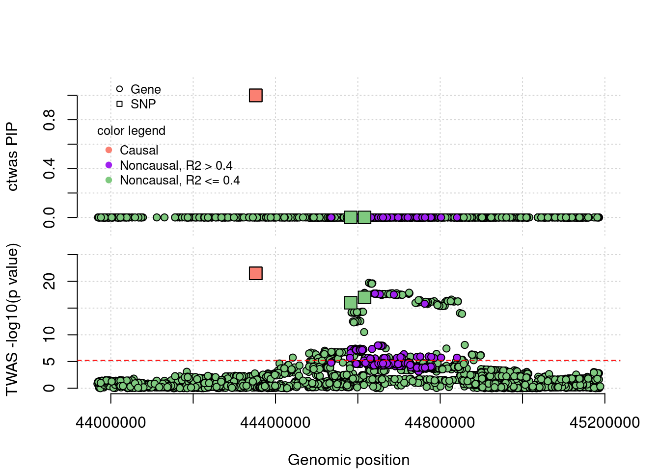

FP example 2

cTWAS avoids the FP error. In this case, the false positive gene (from TWAS) is caused by LD of eQTLs with a causal SNP nearby.

simutag <- "4-1"
a <- plot_region(runtag, simutag, configtag, chr = 5, startpos = 152867774, endpos = 153773088)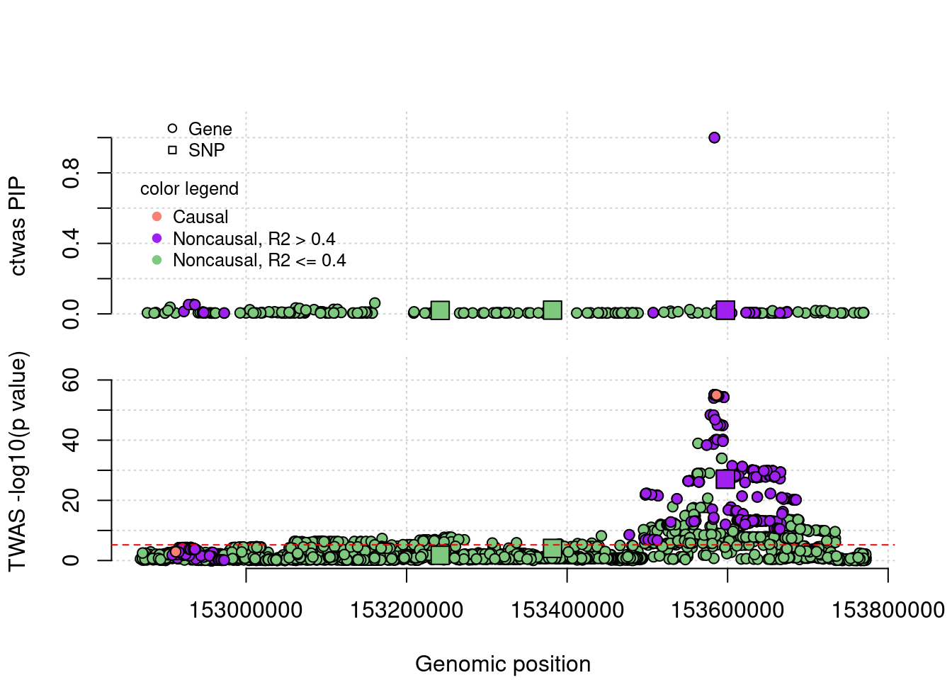

TP example

cTWAS is able to find true positives. This gene has one eQTL, cTWAS choose this gene because it uses a prior favoring genes, it didn't reach significance level by TWAS after bonferron correction.

simutag <- "4-4"
a <- plot_region(runtag, simutag, configtag, chr = 1, startpos = 37549183 , endpos =38731847)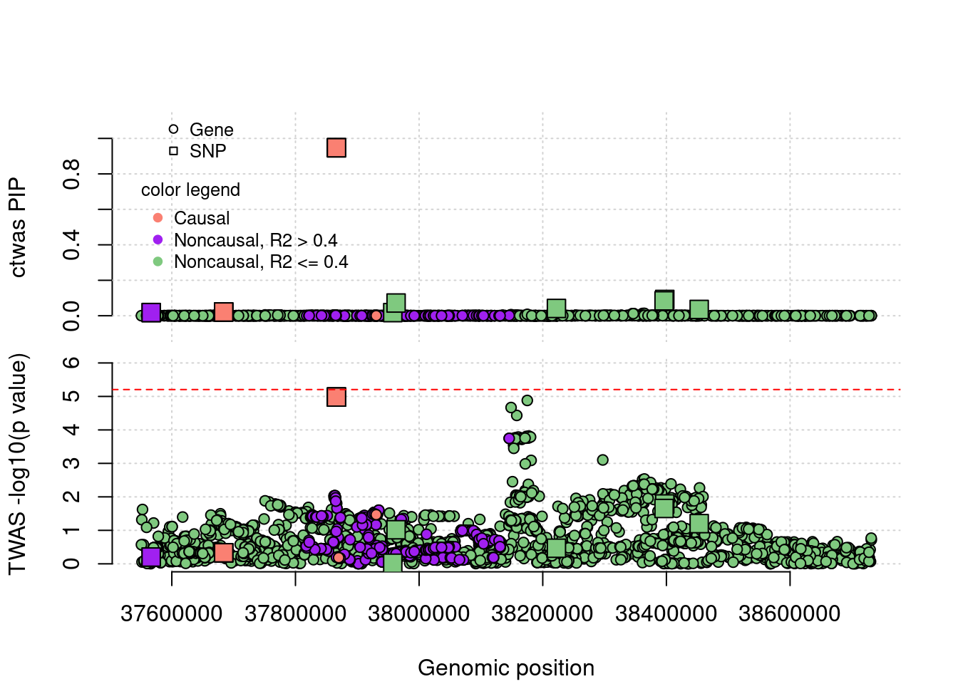

sessionInfo()

R version 3.6.1 (2019-07-05)
Platform: x86_64-pc-linux-gnu (64-bit)
Running under: Scientific Linux 7.4 (Nitrogen)

Matrix products: default
BLAS/LAPACK: /software/openblas-0.2.19-el7-x86_64/lib/libopenblas_haswellp-r0.2.19.so

locale:
 [1] LC_CTYPE=en_US.UTF-8       LC_NUMERIC=C              
 [3] LC_TIME=en_US.UTF-8        LC_COLLATE=en_US.UTF-8    
 [5] LC_MONETARY=en_US.UTF-8    LC_MESSAGES=en_US.UTF-8   
 [7] LC_PAPER=en_US.UTF-8       LC_NAME=C                 
 [9] LC_ADDRESS=C               LC_TELEPHONE=C            
[11] LC_MEASUREMENT=en_US.UTF-8 LC_IDENTIFICATION=C       

attached base packages:
[1] stats     graphics  grDevices utils     datasets  methods   base     

other attached packages:
[1] ggpubr_0.4.0      plotrix_3.7-6     cowplot_1.0.0     ggplot2_3.3.3    
[5] data.table_1.13.2 ctwas_0.1.28     

loaded via a namespace (and not attached):
 [1] Rcpp_1.0.5        lattice_0.20-38   tidyr_1.1.0       rprojroot_1.3-2  
 [5] digest_0.6.20     foreach_1.4.4     utf8_1.1.4        cellranger_1.1.0 
 [9] R6_2.4.0          backports_1.1.4   evaluate_0.14     highr_0.8        
[13] pillar_1.5.1      rlang_0.4.10      readxl_1.3.1      curl_3.3         
[17] car_3.0-5         R.oo_1.22.0       R.utils_2.9.0     Matrix_1.2-18    
[21] rmarkdown_2.9     labeling_0.3      stringr_1.4.0     foreign_0.8-71   
[25] munsell_0.5.0     broom_0.7.5       compiler_3.6.1    httpuv_1.6.1     
[29] xfun_0.24         pkgconfig_2.0.2   htmltools_0.3.6   tidyselect_1.1.0 
[33] gridExtra_2.3     tibble_3.1.0      workflowr_1.6.2   logging_0.10-108 
[37] rio_0.5.16        codetools_0.2-16  fansi_0.4.0       crayon_1.3.4     
[41] dplyr_1.0.5       withr_2.4.1       later_0.8.0       R.methodsS3_1.7.1
[45] grid_3.6.1        gtable_0.3.0      lifecycle_1.0.0   DBI_1.1.0        
[49] git2r_0.26.1      magrittr_1.5      scales_1.1.0      zip_2.0.3        
[53] carData_3.0-2     stringi_1.4.3     debugme_1.1.0     farver_2.1.0     
[57] ggsignif_0.5.0    fs_1.3.1          promises_1.0.1    pgenlibr_0.2     
[61] ellipsis_0.2.0.1  generics_0.0.2    vctrs_0.3.7       openxlsx_4.1.0.1 
[65] iterators_1.0.10  tools_3.6.1       forcats_0.4.0     glue_1.4.2       
[69] purrr_0.3.4       hms_0.5.3         abind_1.4-5       yaml_2.2.0       
[73] colorspace_1.4-1  rstatix_0.7.0     knitr_1.33        haven_2.3.1