Summarize twas
Last updated: 2020-08-04
Checks: 6 1
Knit directory: causal-TWAS/
This reproducible R Markdown analysis was created with workflowr (version 1.6.2). The Checks tab describes the reproducibility checks that were applied when the results were created. The Past versions tab lists the development history.
The R Markdown is untracked by Git. To know which version of the R Markdown file created these results, you’ll want to first commit it to the Git repo. If you’re still working on the analysis, you can ignore this warning. When you’re finished, you can run wflow_publish to commit the R Markdown file and build the HTML.
Great job! The global environment was empty. Objects defined in the global environment can affect the analysis in your R Markdown file in unknown ways. For reproduciblity it’s best to always run the code in an empty environment.
The command set.seed(20191103) was run prior to running the code in the R Markdown file. Setting a seed ensures that any results that rely on randomness, e.g. subsampling or permutations, are reproducible.
Great job! Recording the operating system, R version, and package versions is critical for reproducibility.
Nice! There were no cached chunks for this analysis, so you can be confident that you successfully produced the results during this run.
Great job! Using relative paths to the files within your workflowr project makes it easier to run your code on other machines.
Great! You are using Git for version control. Tracking code development and connecting the code version to the results is critical for reproducibility.
The results in this page were generated with repository version dff432c. See the Past versions tab to see a history of the changes made to the R Markdown and HTML files.
Note that you need to be careful to ensure that all relevant files for the analysis have been committed to Git prior to generating the results (you can use wflow_publish or wflow_git_commit). workflowr only checks the R Markdown file, but you know if there are other scripts or data files that it depends on. Below is the status of the Git repository when the results were generated:
Ignored files:
    Ignored:    .Rhistory
    Ignored:    .Rproj.user/
    Ignored:    code/workflow/.ipynb_checkpoints/
    Ignored:    data/

Untracked files:
    Untracked:  analysis/simulation-multi-ukbchr17to22-gtex.adipose_sa2_v2.Rmd
    Untracked:  code/run_test_mr.ash2s_temp.R

Unstaged changes:
    Modified:   analysis/index.Rmd
    Modified:   analysis/simulation-multi-ukbchr17to22-gtex.adipose.Rmd
    Modified:   analysis/simulation-multi-ukbchr22-gtex.adipose2.Rmd
    Modified:   code/mr.ash2_FBM.R
    Modified:   code/run_simulate_data.R
    Modified:   code/run_test_mr.ash2s.R
    Modified:   code/run_test_susie.R
    Modified:   code/workflow/workflow-ashtest-20200730.ipynb
    Modified:   code/workflow/workflow-ashtest3.ipynb
    Modified:   code/workflow/workflow-ashtest4.ipynb
Note that any generated files, e.g. HTML, png, CSS, etc., are not included in this status report because it is ok for generated content to have uncommitted changes.
There are no past versions. Publish this analysis with wflow_publish() to start tracking its development.
Run simulation 8 times for ukb chr 17 to chr 22 combined. SNPs are downsampled to 1/10, eQTLs defined by FUSION-TWAS (Adipose/GTEx) lasso effect size > 0 were kept, p= 86k, n = 20k.
library(mr.ash.alpha)
library(data.table)
suppressMessages({library(plotly)})
library(tidyr)
library(plyr)
library(stringr)
library(kableExtra)
simdatadir <- "~/causalTWAS/simulations/simulation_ashtest_20200721/"
outputdir <- "~/causalTWAS/simulations/simulation_ashtest_20200721/"
susiedir <- "~/causalTWAS/simulations/simulation_susietest_20200721/"
tags <- paste0('20200721-1-', 1:7)
tagglob <- '20200721-1-*'
tagextr <- '20200721-1-\\d+'
tag2s <- c('zeroes-es', 'zerose-es', 'lassoes-es','lassoes-se')get_files <- function(tag, tag2){
par <- paste0(outputdir, tag, "-mr.ash2s.", tag2, ".param.txt")
rpip <- paste0(outputdir, tag, "-mr.ash2s.", tag2, ".rPIP.txt")
gmrash <- paste0(outputdir, tag, "-mr.ash2s.", tag2, ".expr.txt")
smrash <- paste0(outputdir, tag, "-mr.ash2s.", tag2, ".snp.txt")
ggwas <- paste0(outputdir, tag, ".exprgwas.txt.gz")
sgwas <- paste0(outputdir, tag, ".snpgwas.txt.gz")
gsusie <- paste0(susiedir, tag, ".", tag2, ".L3.susieres.expr.txt")
ssusie <- paste0(susiedir, tag, ".", tag2, ".L3.susieres.snp.txt")
return(tibble::lst(par, rpip, gmrash, ggwas, smrash, sgwas, gsusie, ssusie))
}
get_tags <- function(globpattern, extrpattern, tag2){
lapply(lapply(get_files(globpattern, tag2), Sys.glob), str_extract, pattern = extrpattern)
}Mr.ash2 parameter estimation
Results for 10 simulations runs, using different initiate and update strategy
show_param <- function(tags, tag2){
  f <- lapply(tags, get_files, tag2 = tag2)
  parf <- lapply(f, '[[', "par")
  param <- do.call(rbind, lapply(parf, function(x) t(read.table(x))[2:1,]))
  truth <- param[1:(nrow(param)/2)*2-1,]
  est <- param[1:(nrow(param)/2)*2,]
  outdt <- matrix(0, ncol = 2*ncol(param), nrow = nrow(param)/2)
  outdt[,c(1,3,5,7)] <- truth
  outdt[,c(2,4,6,8)] <- est
  outdt <-cbind(1:nrow(outdt),outdt)
  colnames(outdt) <- c("Simulation#", paste0(rep(c("Truth","Est."),4)))
  knitr::kable(outdt) %>%
  kable_styling("striped") %>%
  add_header_above(c(" " = 1, "Gene.pi1" = 2, "Gene.PVE" = 2, "SNP.pi1" = 2, "SNP.PVE" =2))
}
NULL; expr-snp; expr-snp
show_param(tags, tag2s[1])| Simulation# | Truth | Est. | Truth | Est. | Truth | Est. | Truth | Est. |
|---|---|---|---|---|---|---|---|---|
| 1 | 0.0502117 | 0.0031701 | 0.0066826 | 0.0022282 | 0.0024981 | 0.0017487 | 0.0510701 | 0.0366234 |
| 2 | 0.0502117 | 0.0043097 | 0.0091963 | 0.0003449 | 0.0024981 | 0.0022082 | 0.0437056 | 0.0458391 |
| 3 | 0.0502117 | 0.0247913 | 0.0114728 | 0.0019731 | 0.0024981 | 0.0023113 | 0.0475207 | 0.0306206 |
| 4 | 0.0502117 | 0.0433514 | 0.0114605 | 0.0116073 | 0.0024981 | 0.0027771 | 0.0548585 | 0.0342852 |
| 5 | 0.0502117 | 0.0554445 | 0.0110859 | 0.0148455 | 0.0024981 | 0.0016182 | 0.0478479 | 0.0243124 |
| 6 | 0.0502117 | 0.0202643 | 0.0097170 | 0.0111216 | 0.0024981 | 0.0019085 | 0.0580372 | 0.0339128 |
| 7 | 0.0502117 | 0.0373301 | 0.0111216 | 0.0145758 | 0.0024981 | 0.0018831 | 0.0491958 | 0.0309898 |
NULL; snp-expr; expr-snp
show_param(tags, tag2s[2])| Simulation# | Truth | Est. | Truth | Est. | Truth | Est. | Truth | Est. |
|---|---|---|---|---|---|---|---|---|
| 1 | 0.0502117 | 0.0031701 | 0.0066826 | 0.0022282 | 0.0024981 | 0.0017487 | 0.0510701 | 0.0366234 |
| 2 | 0.0502117 | 0.0043097 | 0.0091963 | 0.0003449 | 0.0024981 | 0.0022082 | 0.0437056 | 0.0458392 |
| 3 | 0.0502117 | 0.0247914 | 0.0114728 | 0.0019731 | 0.0024981 | 0.0023113 | 0.0475207 | 0.0306209 |
| 4 | 0.0502117 | 0.0424709 | 0.0114605 | 0.0118770 | 0.0024981 | 0.0025278 | 0.0548585 | 0.0343060 |
| 5 | 0.0502117 | 0.0558006 | 0.0110859 | 0.0146272 | 0.0024981 | 0.0016143 | 0.0478479 | 0.0242827 |
| 6 | 0.0502117 | 0.0202638 | 0.0097170 | 0.0111219 | 0.0024981 | 0.0019085 | 0.0580372 | 0.0339131 |
| 7 | 0.0502117 | 0.0373297 | 0.0111216 | 0.0145756 | 0.0024981 | 0.0018832 | 0.0491958 | 0.0309887 |
lasso; expr-snp; expr-snp
show_param(tags, tag2s[3])| Simulation# | Truth | Est. | Truth | Est. | Truth | Est. | Truth | Est. |
|---|---|---|---|---|---|---|---|---|
| 1 | 0.0502117 | 0.0031626 | 0.0066826 | 0.0022370 | 0.0024981 | 0.0017442 | 0.0510701 | 0.0372794 |
| 2 | 0.0502117 | 0.0023143 | 0.0091963 | 0.0001921 | 0.0024981 | 0.0019384 | 0.0437056 | 0.0363801 |
| 3 | 0.0502117 | 0.0237669 | 0.0114728 | 0.0018924 | 0.0024981 | 0.0022848 | 0.0475207 | 0.0307098 |
| 4 | 0.0502117 | 0.0159417 | 0.0114605 | 0.0012828 | 0.0024981 | 0.0025405 | 0.0548585 | 0.0483650 |
| 5 | 0.0502117 | 0.0588623 | 0.0110859 | 0.0128581 | 0.0024981 | 0.0015320 | 0.0478479 | 0.0239580 |
| 6 | 0.0502117 | 0.0204854 | 0.0097170 | 0.0109340 | 0.0024981 | 0.0018279 | 0.0580372 | 0.0330261 |
| 7 | 0.0502117 | 0.0397177 | 0.0111216 | 0.0148919 | 0.0024981 | 0.0017947 | 0.0491958 | 0.0375966 |
lasso; expr-snp; snp-expr
show_param(tags, tag2s[4])| Simulation# | Truth | Est. | Truth | Est. | Truth | Est. | Truth | Est. |
|---|---|---|---|---|---|---|---|---|
| 1 | 0.0502117 | 0.0028511 | 0.0066826 | 0.0022522 | 0.0024981 | 0.0014071 | 0.0510701 | 0.0381575 |
| 2 | 0.0502117 | 0.0148369 | 0.0091963 | 0.0061704 | 0.0024981 | 0.0015261 | 0.0437056 | 0.0302851 |
| 3 | 0.0502117 | 0.0392584 | 0.0114728 | 0.0124768 | 0.0024981 | 0.0015233 | 0.0475207 | 0.0255997 |
| 4 | 0.0502117 | 0.0383624 | 0.0114605 | 0.0115444 | 0.0024981 | 0.0018645 | 0.0548585 | 0.0391774 |
| 5 | 0.0502117 | 0.0478061 | 0.0110859 | 0.0156099 | 0.0024981 | 0.0011384 | 0.0478479 | 0.0235886 |
| 6 | 0.0502117 | 0.0225364 | 0.0097170 | 0.0127132 | 0.0024981 | 0.0014313 | 0.0580372 | 0.0308298 |
| 7 | 0.0502117 | 0.0392400 | 0.0111216 | 0.0153121 | 0.0024981 | 0.0015686 | 0.0491958 | 0.0371479 |
Regional mr.ash2s PIP overview
Take simulation 1 (NULL; expr-snp; expr-snp) as examples. We use region size 500kb and PIP cut off at 0.5 for SUSIE.
chrom = 18
f <- get_files(tag= "20200721-1-2" , tag2 = tag2s[1])
allchr <- read.table(f[["rpip"]], header = T)
a <- allchr[allchr["chrom"]==chrom,]
print(paste("plot for chr", chrom))
[1] "plot for chr 18"par(mar=c(5, 4, 4, 6) + 0.1)
with(a, plot(p0, rPIP, col ='salmon', xlab = "position", ylab= "Sum of PIP", type = 'h', lwd = 2))
par(new = T)
with(a, plot(p0, nCausal, pch =19, col = "darkgreen",axes = FALSE, bty = "n", xlab = "", ylab = ""))
axis(side = 4)
mtext(side = 4, line = 3, 'No. causal signals')
legend("topleft",
legend=c("Mr.ASH PIP", "# Causal"),
lty=c(1,0), pch=c(NA, 19), col=c("salmon", "darkgreen"))
grid()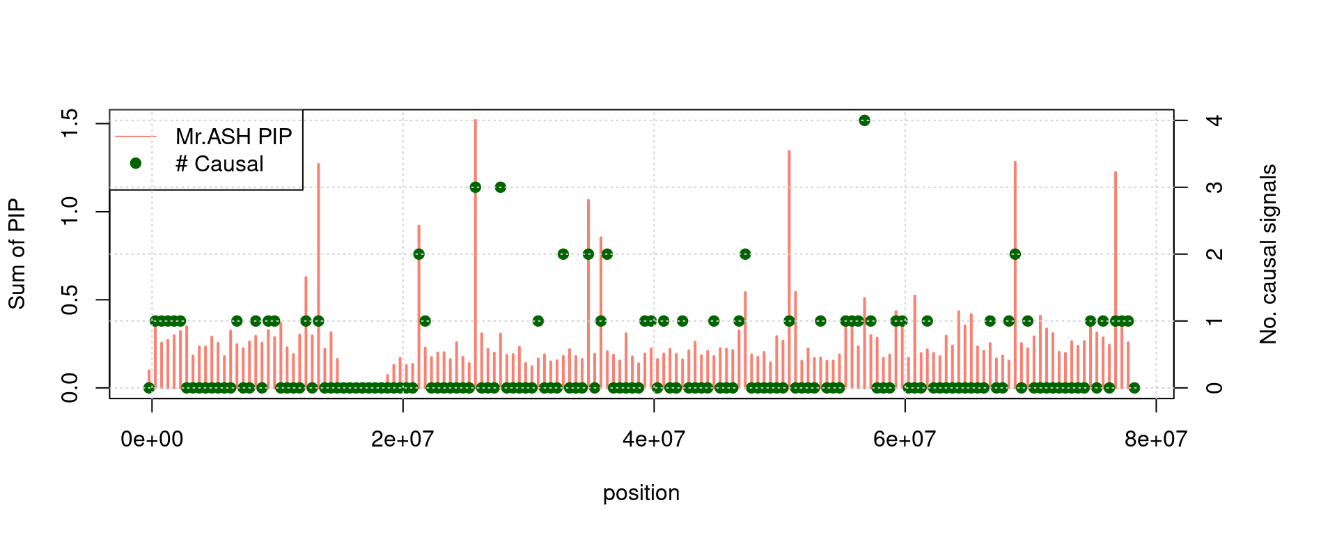
PIP calibration
We run 50 simulations and combine results.
#' s is pip or fdr.
cp_plot <- function(s, ifcausal, mode = c("PIP", "FDR"), main = mode[1]){
  # ifcausal:0,1
  a_bin <- cut(s, breaks= seq(0,1, by=0.1))
  if (mode == "PIP") {
     expected = c(by(s, a_bin, FUN = mean))
     observed = c(by(ifcausal, a_bin, FUN = mean))
  } else if (mode == "FDR"){
     expected = c(by(s, a_bin, FUN = mean))
     observed = 1 - c(by(ifcausal, a_bin, FUN = mean))
  }
  plot(expected, observed, xlim= c(0,1), ylim=c(0,1), pch =19, main = main)
  lines(x = c(0,1), y = c(0,1), col ="red")
}

caliPIP_plot <- function(tags, tag2){
  f <- lapply(tags, get_files, tag2 = tag2)
  mrashf <- lapply(f, '[[', "gmrash")
  names(mrashf) <- tags

  susief <- lapply(f, '[[', "gsusie")
  names(susief) <- tags

  .tagname <- function(x, flist){
    a <- read.table(flist[[x]], header =T)
    a[, "name"] <- paste0(x, ":", a[, "name"])
    a
  }
  mrashres <- do.call(rbind, lapply(tags, .tagname, flist = mrashf))
  susieres <- do.call(rbind, lapply(tags, .tagname, flist = susief))

  res <- merge(mrashres, susieres, by = "name", all = T)

  res <- res[complete.cases(res),]
  res <- rename(res, c("PIP" = "mr.ash_PIP", "pip" = "SUSIE_PIP", "pip.null" = "SUSIE_PIP_null", "pip.w0" = "SUSIE_PIP_w0"))
  par(mfrow=c(1,4), mar=c(5, 6, 4, 1))
  cp_plot(res$mr.ash_PIP, res$ifcausal, main = "Mr.ash PIP")
  cp_plot(res$SUSIE_PIP, res$ifcausal, main = "SUSIE PIP")
  cp_plot(res$SUSIE_PIP_null, res$ifcausal, main = "SUSIE PIP null")
  cp_plot(res$SUSIE_PIP_w0, res$ifcausal, main = "SUSIE PIP weighted null")
}

caliFDR_plot <- function(tags, tag2){

  f <- lapply(tags, get_files, tag2 = tag2)
  gwasf <- lapply(f, '[[', "ggwas")
  names(gwasf) <- tags

  .tagname <- function(x, flist, colnames = NULL){
    a <- read.table(flist[[x]], header =T)
    if (!is.null(colnames)){
      colnames(a) <- colnames
    }
    a[, "name"] <- paste0(x, ":", a[, "name"])
    a
  }

  .addFDR <- function(res){
    res$FDR <- p.adjust(res$PVALUE, method = "fdr")
    res
  }


  gwasres <- do.call(rbind, lapply(lapply(tags, .tagname, flist = gwasf,
                                   colnames =  c("chr", "p0",   "p1", "name",
                                                 "Estimate", "Std.Error", "t-value", "PVALUE")), .addFDR))

  f <- lapply(tags, get_files, tag2 = tag2)
  mrashf <- lapply(f, '[[', "gmrash")
  names(mrashf) <- tags

  susief <- lapply(f, '[[', "gsusie")
  names(susief) <- tags

  .tagname <- function(x, flist){
    a <- read.table(flist[[x]], header =T)
    a[, "name"] <- paste0(x, ":", a[, "name"])
    a
  }
  mrashres <- do.call(rbind, lapply(tags, .tagname, flist = mrashf))
  susieres <- do.call(rbind, lapply(tags, .tagname, flist = susief))

  res <- merge(mrashres, susieres, by = "name", all = T)

  res <- merge(res, gwasres, by = "name", all = T)

  res <- res[complete.cases(res),]

  cp_plot(res$FDR, res$ifcausal, mode ="FDR", main = "TWAS FDR")
  cat("FDR at bonferroni corrected p = 0.05: ", 1 - mean(res[res$PVALUE < 0.05 /dim(res)[1], "ifcausal"]))
}
NULL; expr-snp; expr-snp
tag2 = "zeroes-es"
tags_ext <- Reduce(intersect, get_tags(tagglob, tagextr, tag2 = tag2)['gsusie'])
res <- caliPIP_plot(tags = tags_ext, tag2 = tag2)
Warning in if (mode == "PIP") {: the condition has length > 1 and only the
first element will be used
Warning in if (mode == "PIP") {: the condition has length > 1 and only the
first element will be used
Warning in if (mode == "PIP") {: the condition has length > 1 and only the
first element will be used
Warning in if (mode == "PIP") {: the condition has length > 1 and only the
first element will be used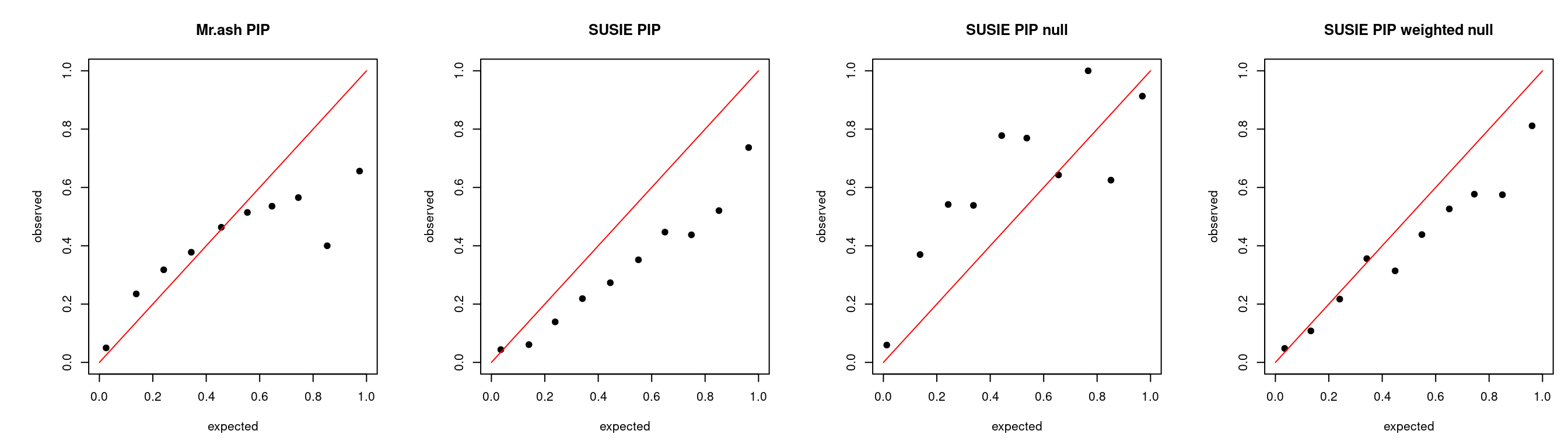
caliFDR_plot(tags = tags_ext, tag2 = tag2)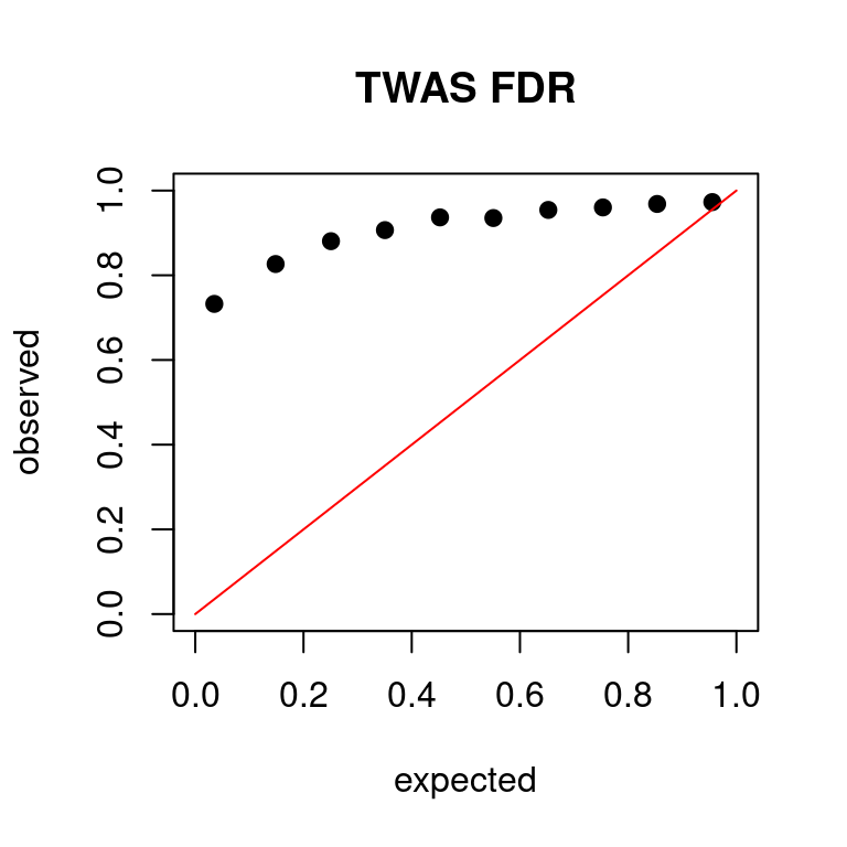
FDR at bonferroni corrected p = 0.05: 0.645933Lasso; expr-snp; expr-snp
caliPIP_plot(tags = tags_ext, tag2 = "lassoes-es")Warning in if (mode == "PIP") {: the condition has length > 1 and only the
first element will be used
Warning in if (mode == "PIP") {: the condition has length > 1 and only the
first element will be used
Warning in if (mode == "PIP") {: the condition has length > 1 and only the
first element will be used
Warning in if (mode == "PIP") {: the condition has length > 1 and only the
first element will be used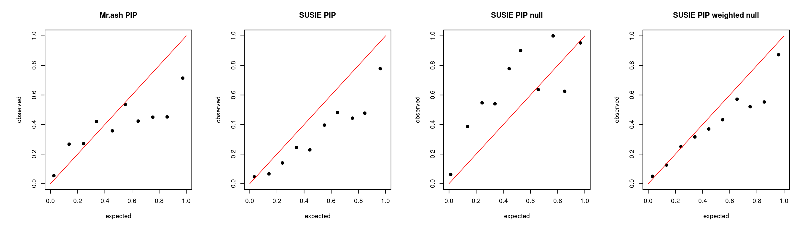
caliFDR_plot(tags = tags_ext, tag2 = "lassoes-es")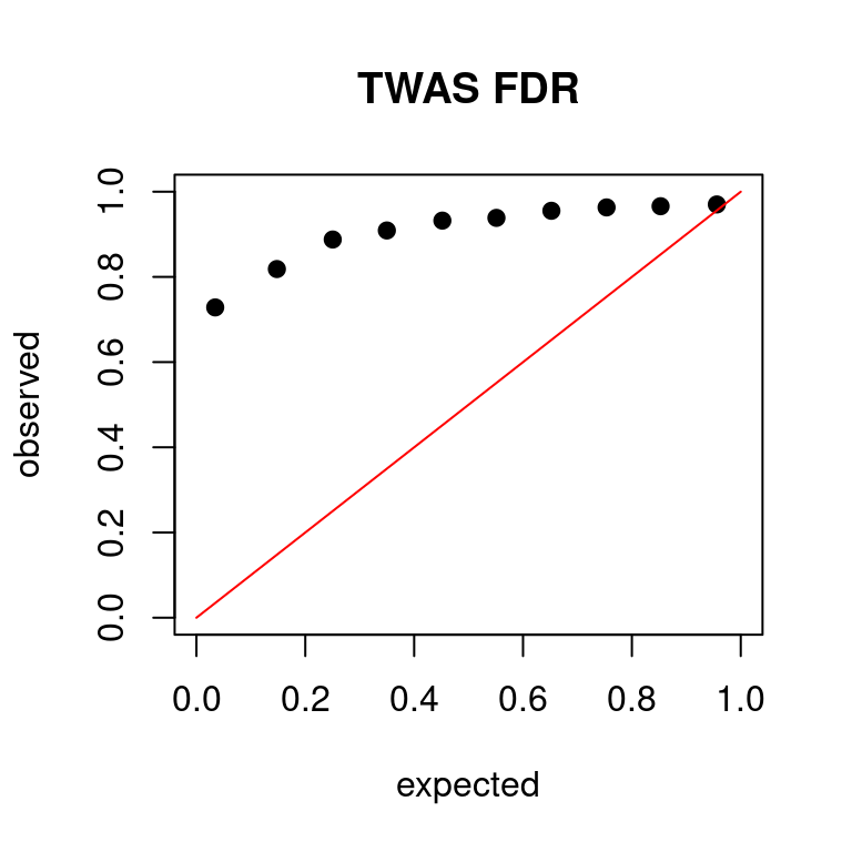
FDR at bonferroni corrected p = 0.05: 0.647343PIP scatter plot
mr.ash2s PIP vs. susie PIP.
scatter_plot_PIP<- function(tags, tag2){
  f <- lapply(tags, get_files, tag2 = tag2)
  mrashf <- lapply(f, '[[', "gmrash")
  names(mrashf) <- tags

  susief <- lapply(f, '[[', "gsusie")
  names(susief) <- tags

  .tagname <- function(x, flist){
    a <- read.table(flist[[x]], header =T)
    a[, "name"] <- paste0(x, ":", a[, "name"])
    a
  }
  mrashres <- do.call(rbind, lapply(tags, .tagname, flist = mrashf))
  susieres <- do.call(rbind, lapply(tags, .tagname, flist = susief))

  res <- merge(mrashres, susieres, by = "name", all = T)

  res <- res[complete.cases(res),]
  res <- rename(res, c("PIP" = "mr.ash_PIP", "pip" = "SUSIE_PIP", "pip.null" = "SUSIE_PIP_null", "pip.w0" = "SUSIE_PIP_w0") )
  res$ifcausal <- mapvalues(res$ifcausal,
          from=c(0,1),
          to=c("Non causal", "Causal"))

  fig1 <- plot_ly(data = res, x = ~ mr.ash_PIP, y = ~ SUSIE_PIP, color = ~ ifcausal,
                 colors = c( "salmon", "darkgreen"))

  fig2 <- plot_ly(data = res, x = ~ mr.ash_PIP, y = ~ SUSIE_PIP_null, color = ~ ifcausal,
                 colors = c( "salmon", "darkgreen"))

  fig3 <- plot_ly(data = res, x = ~ mr.ash_PIP, y = ~ SUSIE_PIP_w0, color = ~ ifcausal,
                 colors = c( "salmon", "darkgreen"))

  fig <- subplot(fig1, fig2, fig3, titleX = TRUE, titleY = T, margin = 0.05)
  fig
}
NULL; expr-snp; expr-snp
scatter_plot_PIP(tags, tag2s[1])Warning: `arrange_()` is deprecated as of dplyr 0.7.0.
Please use `arrange()` instead.
See vignette('programming') for more help
This warning is displayed once every 8 hours.
Call `lifecycle::last_warnings()` to see where this warning was generated.scatter_plot_PIP(tags, tag2s[2])scatter_plot_PIP(tags, tag2s[3])lasso; expr-snp; snp-expr
scatter_plot_PIP(tags, tag2s[4])ROC curve
ROC_plot<- function(tags, tag2){
  f <- lapply(tags, get_files, tag2 = tag2)
  mrashf <- lapply(f, '[[', "gmrash")
  names(mrashf) <- tags

  susief <- lapply(f, '[[', "gsusie")
  names(susief) <- tags

  gwasf <- lapply(f, '[[', "ggwas")
  names(gwasf) <- tags

  .tagname <- function(x, flist, colnames = NULL){
    a <- read.table(flist[[x]], header =T)
    if (!is.null(colnames)){
      colnames(a) <- colnames
    }
    a[, "name"] <- paste0(x, ":", a[, "name"])
    a
  }
  mrashres <- do.call(rbind, lapply(tags, .tagname, flist = mrashf))
  susieres <- do.call(rbind, lapply(tags, .tagname, flist = susief))
  gwasres <- do.call(rbind, lapply(tags, .tagname, flist = gwasf,
                                   colnames =  c("chr", "p0",   "p1", "name", "Estimate", "Std.Error", "t-value", "PVALUE")))

  res <- merge(mrashres, susieres, by = "name", all = T)
  res <- merge(res, gwasres, by = "name", all = T)

  res <- res[complete.cases(res),]
  res <- rename(res, c("PIP" = "mr.ash", "pip" = "SUSIE", "pip.null"= "SUSIE.null", "pip.w0" = "SUSIE.w0", "PVALUE" = "TWAS") )
  res[,"TWAS"] <- -log10(res[, "TWAS"])

  roccolors <-  c("red", "green", "orange", "pink", "blue")
  methods <- c("mr.ash", "SUSIE", "SUSIE.null", "SUSIE.w0", "TWAS")
  plot(0, xlim=c(0,1), ylim=c(0,1), col="white", xlab = "FPR", ylab = "TPR")
  for (i in 1:length(methods)){
    method <- methods[i]
    bordered <- res[order(res[,method]),]
    actuals <- bordered$ifcausal == 1
    sens <- (sum(actuals) - cumsum(actuals))/sum(actuals)
    spec <- cumsum(!actuals)/sum(!actuals)
    lines(1 - spec, sens, type = "l", col = roccolors[i])
    abline(c(0,0),c(1,1))
    auc <- sum(spec*diff(c(0, 1 - sens)))
    cat("AUC for ", method, ": ", auc)
  }
  legend(0.6,0.3, legend= methods, col=roccolors, lty=1, cex=0.5 )
  grid()
}
NULL; expr-snp; expr-snp
tags <- paste0('20200721-1-', c(2,4:9))
ROC_plot(tags, tag2s[2])
AUC for mr.ash : 0.6894131AUC for SUSIE : 0.6824739AUC for SUSIE.null : 0.6762515AUC for SUSIE.w0 : 0.6835701AUC for TWAS : 0.7488581NULL; snp-expr; expr-snp
ROC_plot(tags, tag2s[2])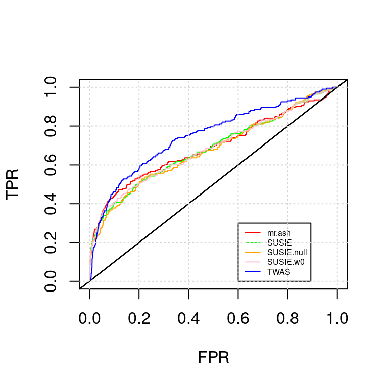
AUC for mr.ash : 0.6894131AUC for SUSIE : 0.6824739AUC for SUSIE.null : 0.6762515AUC for SUSIE.w0 : 0.6835701AUC for TWAS : 0.7488581lasso; expr-snp; expr-snp
ROC_plot(tags, tag2s[3])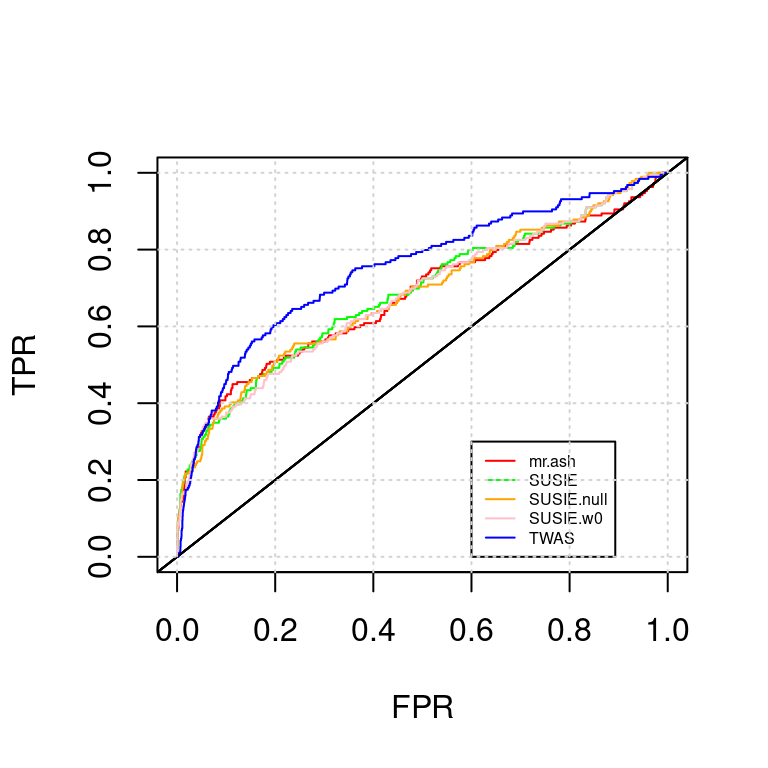
AUC for mr.ash : 0.6778905AUC for SUSIE : 0.6857911AUC for SUSIE.null : 0.6818999AUC for SUSIE.w0 : 0.6799617AUC for TWAS : 0.7489982lasso; expr-snp; snp-expr
ROC_plot(tags, tag2s[4])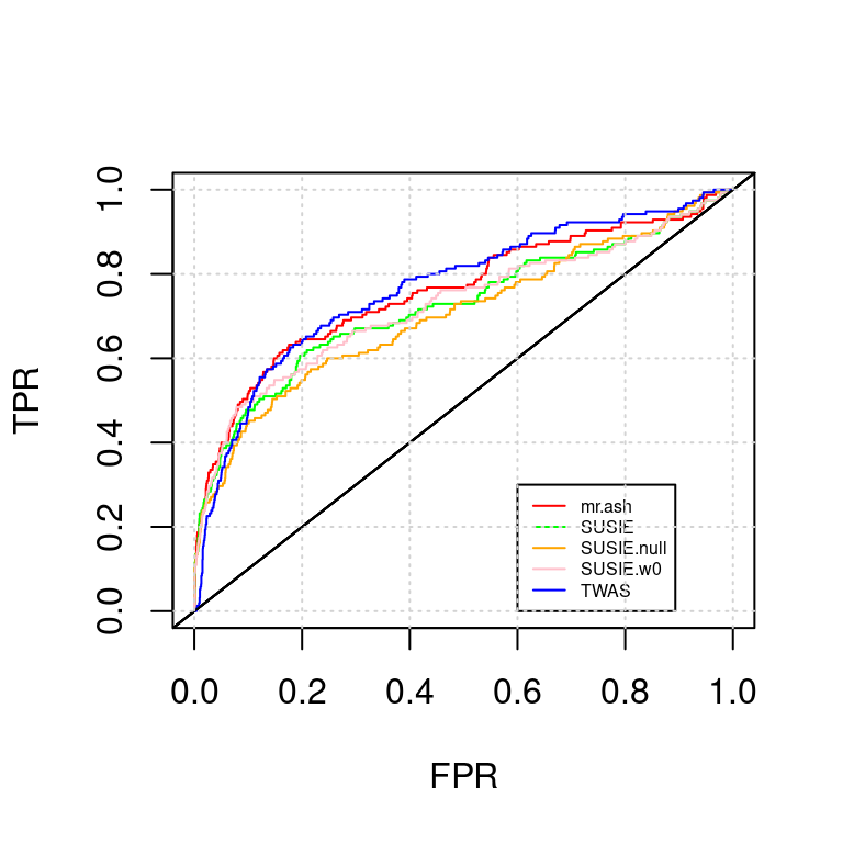
AUC for mr.ash : 0.7589313AUC for SUSIE : 0.7235847AUC for SUSIE.null : 0.7043028AUC for SUSIE.w0 : 0.7258811AUC for TWAS : 0.768614
sessionInfo()R version 3.5.1 (2018-07-02)
Platform: x86_64-pc-linux-gnu (64-bit)
Running under: Scientific Linux 7.4 (Nitrogen)
Matrix products: default
BLAS/LAPACK: /software/openblas-0.2.19-el7-x86_64/lib/libopenblas_haswellp-r0.2.19.so
locale:
[1] LC_CTYPE=en_US.UTF-8 LC_NUMERIC=C
[3] LC_TIME=en_US.UTF-8 LC_COLLATE=en_US.UTF-8
[5] LC_MONETARY=en_US.UTF-8 LC_MESSAGES=en_US.UTF-8
[7] LC_PAPER=en_US.UTF-8 LC_NAME=C
[9] LC_ADDRESS=C LC_TELEPHONE=C
[11] LC_MEASUREMENT=en_US.UTF-8 LC_IDENTIFICATION=C
attached base packages:
[1] stats graphics grDevices utils datasets methods base
other attached packages:
[1] kableExtra_1.1.0 stringr_1.4.0 plyr_1.8.6
[4] tidyr_0.8.3 plotly_4.9.2.9000 ggplot2_3.3.1
[7] data.table_1.12.7 mr.ash.alpha_0.1-34
loaded via a namespace (and not attached):
[1] tidyselect_1.1.0 purrr_0.3.4 lattice_0.20-38
[4] colorspace_1.3-2 vctrs_0.3.1 generics_0.0.2
[7] htmltools_0.3.6 viridisLite_0.3.0 yaml_2.2.0
[10] rlang_0.4.6 later_0.7.5 pillar_1.4.4
[13] glue_1.4.1 withr_2.1.2 lifecycle_0.2.0
[16] munsell_0.5.0 gtable_0.2.0 workflowr_1.6.2
[19] rvest_0.3.2 htmlwidgets_1.3 evaluate_0.12
[22] knitr_1.20 crosstalk_1.0.0 httpuv_1.4.5
[25] highr_0.7 Rcpp_1.0.4.6 xtable_1.8-3
[28] readr_1.3.1 promises_1.0.1 scales_1.0.0
[31] backports_1.1.2 webshot_0.5.1 jsonlite_1.6.1
[34] mime_0.6 fs_1.3.1 hms_0.4.2
[37] digest_0.6.25 stringi_1.3.1 shiny_1.2.0
[40] dplyr_1.0.0 grid_3.5.1 rprojroot_1.3-2
[43] tools_3.5.1 magrittr_1.5 lazyeval_0.2.1
[46] tibble_3.0.1 crayon_1.3.4 pkgconfig_2.0.2
[49] ellipsis_0.3.1 Matrix_1.2-15 xml2_1.2.0
[52] rmarkdown_1.10 httr_1.4.1 rstudioapi_0.11
[55] R6_2.3.0 git2r_0.26.1 compiler_3.5.1