SuSiE RSS convergence problem
Yuxin Zou
3/6/2021
Last updated: 2021-03-06
Checks: 7 0
Knit directory: dsc_susierss/
This reproducible R Markdown analysis was created with workflowr (version 1.6.2). The Checks tab describes the reproducibility checks that were applied when the results were created. The Past versions tab lists the development history.
Great! Since the R Markdown file has been committed to the Git repository, you know the exact version of the code that produced these results.
Great job! The global environment was empty. Objects defined in the global environment can affect the analysis in your R Markdown file in unknown ways. For reproduciblity it’s best to always run the code in an empty environment.
The command set.seed(20210220) was run prior to running the code in the R Markdown file. Setting a seed ensures that any results that rely on randomness, e.g. subsampling or permutations, are reproducible.
Great job! Recording the operating system, R version, and package versions is critical for reproducibility.
Nice! There were no cached chunks for this analysis, so you can be confident that you successfully produced the results during this run.
Great job! Using relative paths to the files within your workflowr project makes it easier to run your code on other machines.
Great! You are using Git for version control. Tracking code development and connecting the code version to the results is critical for reproducibility.
The results in this page were generated with repository version a100dd6. See the Past versions tab to see a history of the changes made to the R Markdown and HTML files.
Note that you need to be careful to ensure that all relevant files for the analysis have been committed to Git prior to generating the results (you can use wflow_publish or wflow_git_commit). workflowr only checks the R Markdown file, but you know if there are other scripts or data files that it depends on. Below is the status of the Git repository when the results were generated:
Ignored files:
    Ignored:    .DS_Store
    Ignored:    .Rhistory
    Ignored:    .Rproj.user/

Untracked files:
    Untracked:  data/susie_convergence_problem.rds

Unstaged changes:
    Modified:   analysis/index.Rmd
    Deleted:    genotype_dir
Note that any generated files, e.g. HTML, png, CSS, etc., are not included in this status report because it is ok for generated content to have uncommitted changes.
These are the previous versions of the repository in which changes were made to the R Markdown (analysis/susie_convergence_problem.Rmd) and HTML (docs/susie_convergence_problem.html) files. If you’ve configured a remote Git repository (see ?wflow_git_remote), click on the hyperlinks in the table below to view the files as they were in that past version.
| File | Version | Author | Date | Message |
|---|---|---|---|---|
| Rmd | a100dd6 | zouyuxin | 2021-03-06 | wflow_publish(“analysis/susie_convergence_problem.Rmd”) |
| html | aa199f5 | zouyuxin | 2021-03-06 | Build site. |
| Rmd | 38bddb8 | zouyuxin | 2021-03-06 | wflow_publish(“analysis/susie_convergence_problem.Rmd”) |
| html | 5abf209 | zouyuxin | 2021-03-06 | Build site. |
| Rmd | 311e2c9 | zouyuxin | 2021-03-06 | wflow_publish(“analysis/susie_convergence_problem.Rmd”) |
| html | 9c68be0 | zouyuxin | 2021-03-06 | Build site. |
| Rmd | 8aa8c36 | zouyuxin | 2021-03-06 | wflow_publish(“analysis/susie_convergence_problem.Rmd”) |
We observe the convergence problem for SuSiE in simulation. We illustrate 2 data here.
library(susieR)
dat = readRDS('data/susie_convergence_problem.rds')
Data 1
The region contains 1001 SNPs. There are two causals at 234, 287.
d1 = dat$d1
b = d1$true_coef
idx = which(b!=0)

par(mfrow=c(1,2))
plot(d1$z, pch = 16, xlab = 'SNPs', ylab = 'z')
points(idx, d1$z[idx], col='red', pch = 16)
log10p = -log10(pnorm(-abs(d1$z))*2)
plot(log10p, pch = 16, xlab = 'SNPs', ylab = '-log10 p value')
points(idx, log10p[idx], col='red', pch = 16)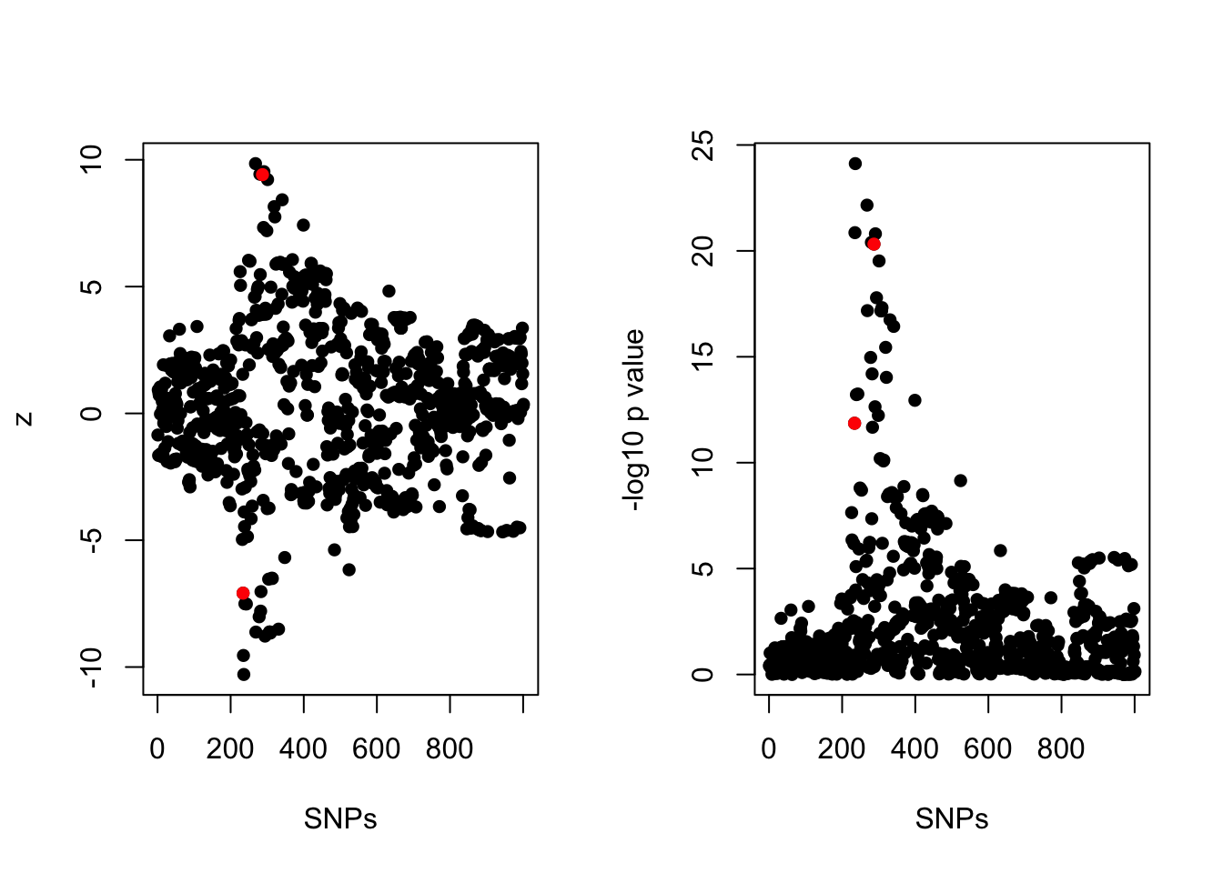
| Version | Author | Date |
|---|---|---|
| 9c68be0 | zouyuxin | 2021-03-06 |
The SNP with strongest marginal association is 236. The correlation between causal SNPs and top SNP is
d1$ld[c(234, 236, 287), c(234, 236, 287)] V234 V236 V287
[1,] 1.0000000 0.56423775 0.53418375
[2,] 0.5642378 1.00000000 -0.03744934
[3,] 0.5341837 -0.03744934 1.00000000Using L = 3, the susie model gives 3 CSs. (I used susie_suff_stat, which gives the same result as susie.)
f1 = susie_suff_stat(XtX = d1$XtX, Xty = d1$Xty, yty = d1$yty, n = d1$n, L=3, track_fit = T)
susie_plot(f1, y='PIP', b=b, add_legend = T, main=paste0('ELBO: ', round(susie_get_objective(f1), 4)))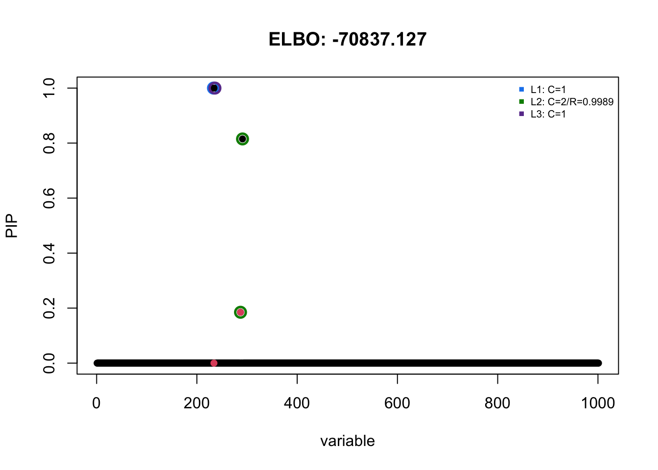
| Version | Author | Date |
|---|---|---|
| 9c68be0 | zouyuxin | 2021-03-06 |
summary(f1)
Variables in credible sets:

 variable variable_prob cs
      233     1.0000000  3
      236     1.0000000  1
      291     0.8150868  2
      287     0.1849131  2

Credible sets summary:

 cs cs_log10bf cs_avg_r2 cs_min_r2 variable
  1   30.80784 1.0000000 1.0000000      236
  3   31.30944 1.0000000 1.0000000      233
  2   61.20570 0.9989095 0.9978195  287,291
The SNPs in CS1 and CS3 are partially correlated with SNP 234. The correlation between them is
d1$ld[c(233, 234, 236), c(233, 234, 236)] V233 V234 V236
[1,] 1.0000000 0.5996649 -0.2407775
[2,] 0.5996649 1.0000000 0.5642378
[3,] -0.2407775 0.5642378 1.0000000susie_plot_iteration(f1, L=3, 'assets/susie_convergence_problem/susie_convergence_problem_d1_f1', pos=c(233, 234, 236, 287, 291))| variable | 1 | 2 | 3 | 4 | 5 |
|---|---|---|---|---|---|
| SNP | 233 | 234 | 236 | 287 | 291 |

Using L = 2, we find the correct CSs, and the ELBO is larger.
f2 = susie_suff_stat(XtX = d1$XtX, Xty = d1$Xty, yty = d1$yty, n = d1$n, L=2, track_fit = T)
susie_plot(f2, y='PIP', b=b, add_legend = T, main=paste0('ELBO: ', round(susie_get_objective(f2), 3)))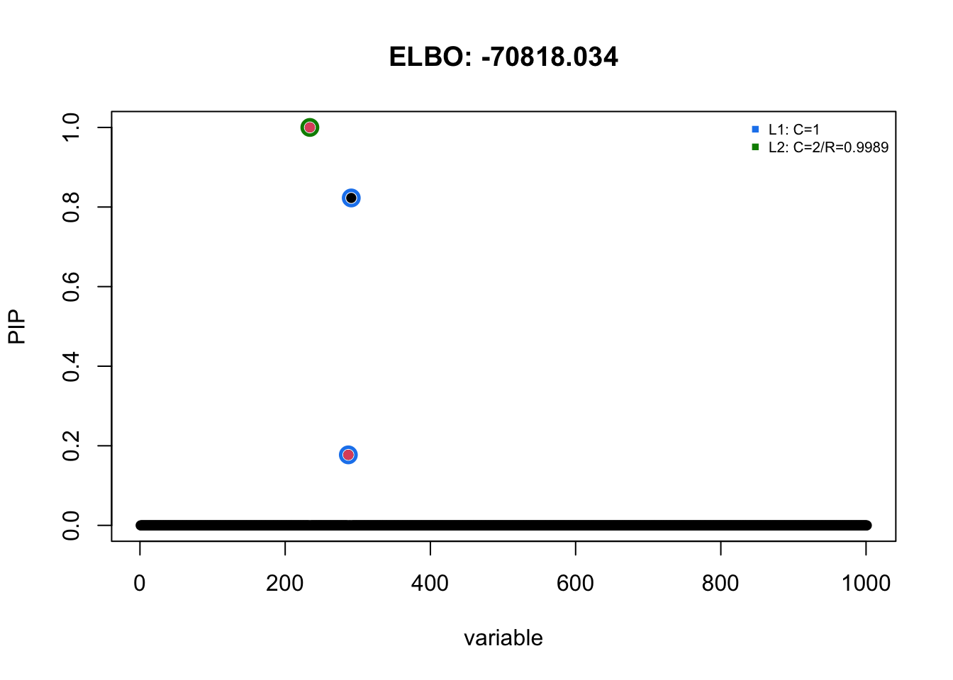
| Version | Author | Date |
|---|---|---|
| 9c68be0 | zouyuxin | 2021-03-06 |
susie_plot_iteration(f2, L=2, 'assets/susie_convergence_problem/susie_convergence_problem_d1_f2', pos=c(233, 234, 236, 287, 291))
Data 2
The region contains 1001 SNPs. There are three causals at 252, 340, 375.
d2 = dat$d2
b = d2$true_coef
idx = which(b!=0)

par(mfrow=c(1,2))
plot(d2$z, pch = 16, xlab = 'SNPs', ylab = 'z')
points(idx, d2$z[idx], col='red', pch = 16)
log10p = -log10(pnorm(-abs(d2$z))*2)
plot(log10p, pch = 16, xlab = 'SNPs', ylab = '-log10 p value')
points(idx, log10p[idx], col='red', pch = 16)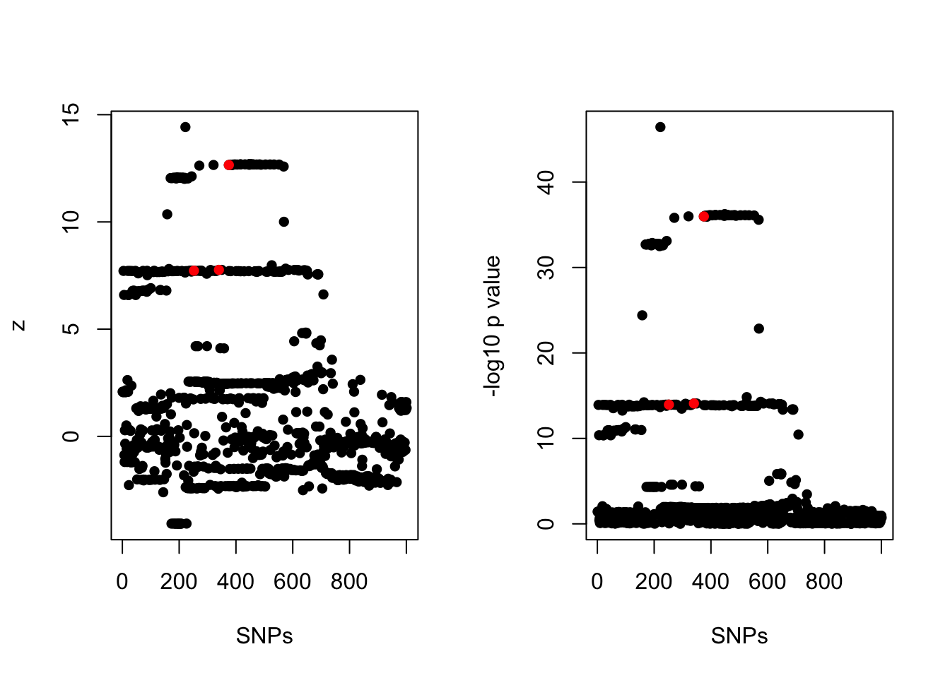
| Version | Author | Date |
|---|---|---|
| 9c68be0 | zouyuxin | 2021-03-06 |
The SNP with strongest marginal association is 222. The correlation between causal SNPs and top SNP is
d2$ld[c(222, idx), c(222, idx)] V222 V252 V340 V375
[1,] 1.0000000 0.5508992 0.55055773 0.79251604
[2,] 0.5508992 1.0000000 0.99949772 -0.01428270
[3,] 0.5505577 0.9994977 1.00000000 -0.01412418
[4,] 0.7925160 -0.0142827 -0.01412418 1.00000000Using L = 10, the susie model gives 1 CS.
f3 = susie_suff_stat(XtX = d2$XtX, Xty = d2$Xty, yty = d2$yty, n = d2$n, L=10, track_fit = T)
susie_plot(f3, y='PIP', b=b, add_legend = T, main=paste0('ELBO: ', round(susie_get_objective(f3), 4)))
| Version | Author | Date |
|---|---|---|
| 9c68be0 | zouyuxin | 2021-03-06 |
It identifies the top SNP.
susie_plot_iteration(f3, L=10, 'assets/susie_convergence_problem/susie_convergence_problem_d2_f3', pos=c(222, idx))
Using L = 3, it converges to the same solution as L = 10.
f4 = susie_suff_stat(XtX = d2$XtX, Xty = d2$Xty, yty = d2$yty, n = d2$n, L=3, track_fit = T,
                     estimate_residual_variance = T, estimate_prior_variance = T)
susie_plot(f4, y='PIP', b=b, add_legend = T, main=paste0('ELBO: ', round(susie_get_objective(f4), 4)))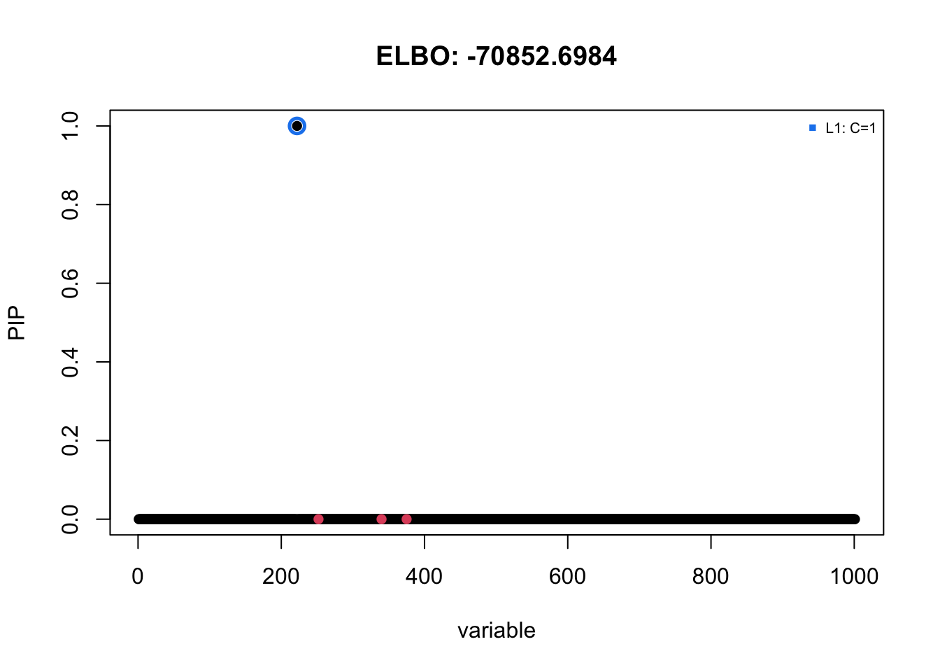
| Version | Author | Date |
|---|---|---|
| 9c68be0 | zouyuxin | 2021-03-06 |
We initialize at the truth,
beta_val = b[idx]
sinit = susieR::susie_init_coef(idx, beta_val, length(b))
finittrue = susie_suff_stat(XtX = d2$XtX, Xty = d2$Xty, yty = d2$yty, n = d2$n, track_fit = T, s_init = sinit,
                            estimate_residual_variance = T,estimate_prior_variance = TRUE, max_iter = 200)
susie_plot(finittrue, y='PIP', b=b, add_legend = T, main=paste0('ELBO: ', round(susie_get_objective(finittrue), 4)))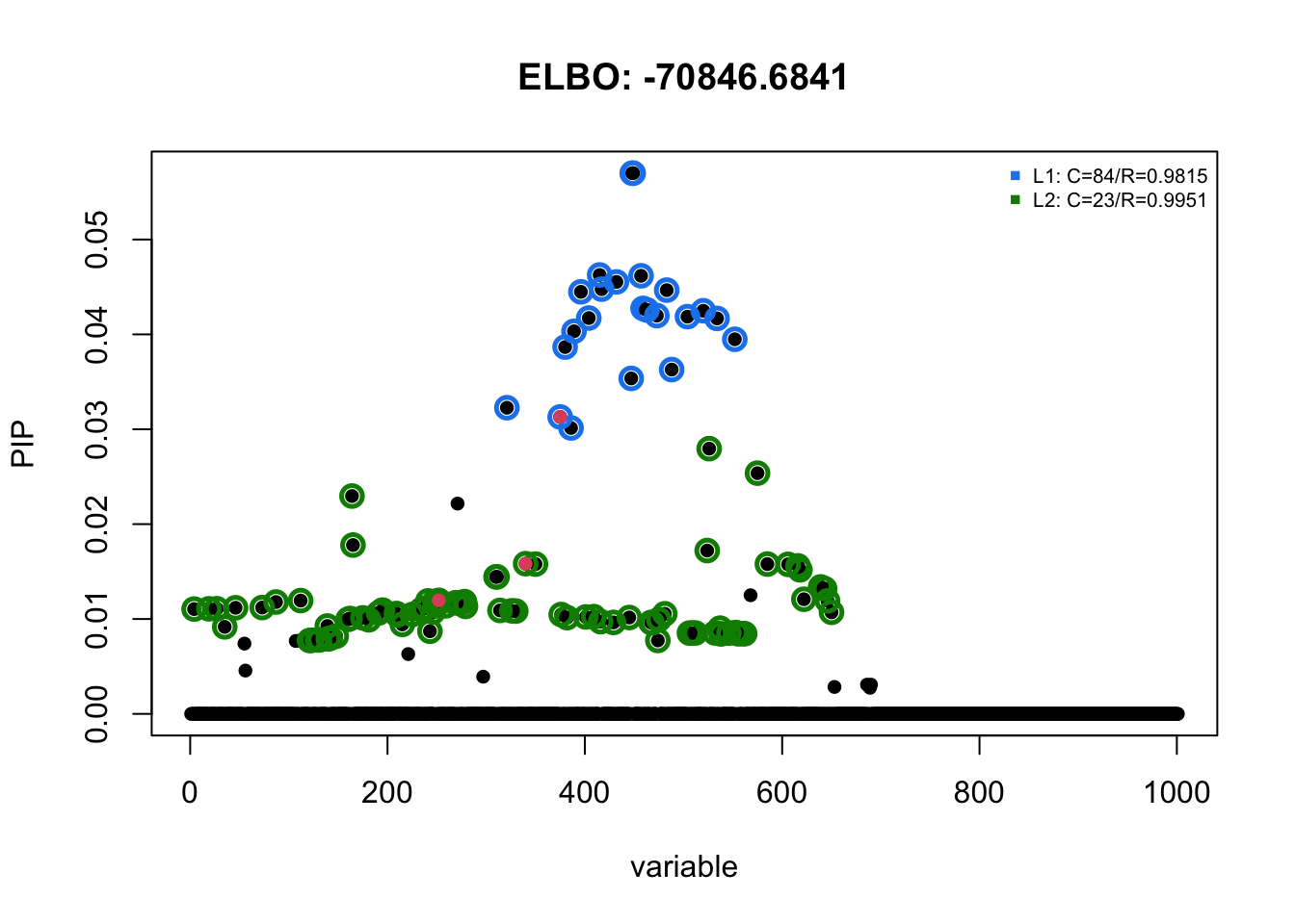
| Version | Author | Date |
|---|---|---|
| 9c68be0 | zouyuxin | 2021-03-06 |
sessionInfo()R version 4.0.3 (2020-10-10)
Platform: x86_64-apple-darwin17.0 (64-bit)
Running under: macOS Big Sur 10.16
Matrix products: default
BLAS: /Library/Frameworks/R.framework/Versions/4.0/Resources/lib/libRblas.dylib
LAPACK: /Library/Frameworks/R.framework/Versions/4.0/Resources/lib/libRlapack.dylib
locale:
[1] en_US.UTF-8/en_US.UTF-8/en_US.UTF-8/C/en_US.UTF-8/en_US.UTF-8
attached base packages:
[1] stats graphics grDevices utils datasets methods base
other attached packages:
[1] susieR_0.10.0 workflowr_1.6.2
loaded via a namespace (and not attached):
[1] Rcpp_1.0.6 plyr_1.8.6 pillar_1.4.7 compiler_4.0.3
[5] later_1.1.0.1 git2r_0.27.1 tools_4.0.3 digest_0.6.27
[9] evaluate_0.14 lifecycle_1.0.0 tibble_3.0.6 gtable_0.3.0
[13] lattice_0.20-41 pkgconfig_2.0.3 rlang_0.4.10 Matrix_1.2-18
[17] yaml_2.2.1 xfun_0.19 stringr_1.4.0 dplyr_1.0.2
[21] knitr_1.30 generics_0.1.0 fs_1.5.0 vctrs_0.3.6
[25] tidyselect_1.1.0 rprojroot_2.0.2 grid_4.0.3 reshape_0.8.8
[29] glue_1.4.2 R6_2.5.0 rmarkdown_2.5 purrr_0.3.4
[33] ggplot2_3.3.3 magrittr_2.0.1 whisker_0.4 scales_1.1.1
[37] promises_1.1.1 ellipsis_0.3.1 htmltools_0.5.0 colorspace_2.0-0
[41] httpuv_1.5.4 stringi_1.5.3 munsell_0.5.0 crayon_1.4.1