EM vs. SCD in a small, simulated data set
Peter Carbonetto
Last updated: 2021-05-06
Checks: 7 0
Knit directory: fastTopics-experiments/analysis/
This reproducible R Markdown analysis was created with workflowr (version 1.6.2.9000). The Checks tab describes the reproducibility checks that were applied when the results were created. The Past versions tab lists the development history.
Great! Since the R Markdown file has been committed to the Git repository, you know the exact version of the code that produced these results.
Great job! The global environment was empty. Objects defined in the global environment can affect the analysis in your R Markdown file in unknown ways. For reproduciblity it’s best to always run the code in an empty environment.
The command set.seed(1) was run prior to running the code in the R Markdown file. Setting a seed ensures that any results that rely on randomness, e.g. subsampling or permutations, are reproducible.
Great job! Recording the operating system, R version, and package versions is critical for reproducibility.
Nice! There were no cached chunks for this analysis, so you can be confident that you successfully produced the results during this run.
Great job! Using relative paths to the files within your workflowr project makes it easier to run your code on other machines.
Great! You are using Git for version control. Tracking code development and connecting the code version to the results is critical for reproducibility.
The results in this page were generated with repository version 4d9c370. See the Past versions tab to see a history of the changes made to the R Markdown and HTML files.
Note that you need to be careful to ensure that all relevant files for the analysis have been committed to Git prior to generating the results (you can use wflow_publish or wflow_git_commit). workflowr only checks the R Markdown file, but you know if there are other scripts or data files that it depends on. Below is the status of the Git repository when the results were generated:
Ignored files:
    Ignored:    analysis/.sos/
    Ignored:    data/20news-bydate/
    Ignored:    data/droplet.RData
    Ignored:    data/nips_1-17.mat
    Ignored:    data/pbmc_68k.RData
    Ignored:    output/droplet/fits-droplet.RData
    Ignored:    output/newsgroups/fits-newsgroups.RData
    Ignored:    output/nips/fits-nips.RData
    Ignored:    output/pbmc68k/fits-pbmc68k.RData

Untracked files:
    Untracked:  plots/

Unstaged changes:
    Modified:   analysis/temp.R
Note that any generated files, e.g. HTML, png, CSS, etc., are not included in this status report because it is ok for generated content to have uncommitted changes.
These are the previous versions of the repository in which changes were made to the R Markdown (analysis/smallsim.Rmd) and HTML (docs/smallsim.html) files. If you’ve configured a remote Git repository (see ?wflow_git_remote), click on the hyperlinks in the table below to view the files as they were in that past version.
| File | Version | Author | Date | Message |
|---|---|---|---|---|
| Rmd | 4d9c370 | Peter Carbonetto | 2021-05-06 | workflowr::wflow_publish(“smallsim.Rmd”) |
| Rmd | 1e58fea | Peter Carbonetto | 2021-04-06 | Revised title in smallsim demo. |
| Rmd | b1c94ad | Peter Carbonetto | 2021-03-19 | Added scd and mu updates to scd_vs_ccd.R. |
| html | aa89a24 | Peter Carbonetto | 2021-03-12 | Created PDF for last plot in smallsim example. |
| Rmd | 1a7515d | Peter Carbonetto | 2021-03-12 | workflowr::wflow_publish(“smallsim.Rmd”) |
| html | 311659c | Peter Carbonetto | 2021-03-12 | Added LDA results for second “smallsim” example. |
| Rmd | 4d2058f | Peter Carbonetto | 2021-03-12 | workflowr::wflow_publish(“smallsim.Rmd”) |
| Rmd | 74d9a5f | Peter Carbonetto | 2021-03-11 | Added code for running LDA on second simulated data set in smallsim.Rmd. |
| Rmd | 1efb089 | Peter Carbonetto | 2021-03-11 | Made improvements to plots in smallsim demo. |
| html | be1f9a4 | Peter Carbonetto | 2021-03-11 | Added LDA fits to first simulated data set in smallsim demo. |
| Rmd | 7f0bc89 | Peter Carbonetto | 2021-03-11 | workflowr::wflow_publish(“smallsim.Rmd”, verbose = TRUE) |
| Rmd | 509961e | Peter Carbonetto | 2021-03-11 | Implemented plotting functions for smallsim demo. |
| Rmd | 0526659 | Peter Carbonetto | 2021-03-10 | Added exploratory scripts smallsimlda.R and smallsimlda2.R. |
| html | daf189c | Peter Carbonetto | 2021-03-09 | Build site. |
| Rmd | 1b18e2d | Peter Carbonetto | 2021-03-09 | workflowr::wflow_publish(“smallsim.Rmd”) |
| html | 47ed425 | Peter Carbonetto | 2021-03-09 | Added KKT residual plots to “smallsim” example. |
| Rmd | eb495f3 | Peter Carbonetto | 2021-03-09 | workflowr::wflow_publish(“smallsim.Rmd”) |
| html | 907addd | Peter Carbonetto | 2021-03-08 | Added more detail to some of the scatterplots in the “smallsim” demo. |
| Rmd | c183922 | Peter Carbonetto | 2021-03-08 | workflowr::wflow_publish(“smallsim.Rmd”) |
| html | 300faac | Peter Carbonetto | 2021-03-08 | Build site. |
| Rmd | 858b366 | Peter Carbonetto | 2021-03-08 | workflowr::wflow_publish(“smallsim.Rmd”) |
| html | 87ef32e | Peter Carbonetto | 2021-03-08 | Added some more plots to smallsim demo. |
| Rmd | c4b4f75 | Peter Carbonetto | 2021-03-08 | workflowr::wflow_publish(“smallsim.Rmd”) |
| html | a967f97 | Peter Carbonetto | 2021-03-08 | Fixed axis label. |
| Rmd | be1777b | Peter Carbonetto | 2021-03-08 | workflowr::wflow_publish(“smallsim.Rmd”) |
| html | 1838ec8 | Peter Carbonetto | 2021-03-08 | Made small change to the plots in the “smallsim” demo. |
| Rmd | eb2f21d | Peter Carbonetto | 2021-03-08 | workflowr::wflow_publish(“smallsim.Rmd”) |
| html | 8e406ad | Peter Carbonetto | 2021-03-07 | Added introductory text to “smallsim” demo. |
| Rmd | bf10490 | Peter Carbonetto | 2021-03-07 | workflowr::wflow_publish(“smallsim.Rmd”) |
| html | 50f34a9 | Peter Carbonetto | 2021-03-07 | Added explanatory text to “smallsim” example. |
| Rmd | f5516ac | Peter Carbonetto | 2021-03-07 | workflowr::wflow_publish(“smallsim.Rmd”) |
| html | 1185ab4 | Peter Carbonetto | 2021-03-07 | Revised the progress plots in the “smallsim” demo. |
| Rmd | f783c31 | Peter Carbonetto | 2021-03-07 | workflowr::wflow_publish(“smallsim.Rmd”) |
| html | 7e3d55b | Peter Carbonetto | 2021-03-07 | Adjusted parameters for second simulation in “smallsim” demo. |
| Rmd | 6e8a2c4 | Peter Carbonetto | 2021-03-07 | workflowr::wflow_publish(“smallsim.Rmd”) |
| html | 913316c | Peter Carbonetto | 2021-03-07 | Added structure plots to “smallsim” demo. |
| Rmd | b9fac71 | Peter Carbonetto | 2021-03-07 | workflowr::wflow_publish(“smallsim.Rmd”) |
| Rmd | 01898db | Peter Carbonetto | 2021-03-06 | Added some text to smallsim.Rmd. |
| html | 51c5321 | Peter Carbonetto | 2021-03-06 | Made some improvements to “smallsim” demo. |
| Rmd | 5983a39 | Peter Carbonetto | 2021-03-06 | workflowr::wflow_publish(“smallsim.Rmd”) |
| Rmd | eff0954 | Peter Carbonetto | 2021-03-06 | Added some explanatory text to smallsim.Rmd. |
| html | eff0954 | Peter Carbonetto | 2021-03-06 | Added some explanatory text to smallsim.Rmd. |
| html | 59a8594 | Peter Carbonetto | 2021-03-05 | Revised the simulations slightly. |
| Rmd | 1a59342 | Peter Carbonetto | 2021-03-05 | workflowr::wflow_publish(“smallsim.Rmd”) |
| html | ffad471 | Peter Carbonetto | 2021-03-05 | Build site. |
| Rmd | cfc44e5 | Peter Carbonetto | 2021-03-05 | workflowr::wflow_publish(“smallsim.Rmd”) |
| html | 52759e5 | Peter Carbonetto | 2021-03-05 | Added first simulation to “smallsim” demo. |
| Rmd | fe510f0 | Peter Carbonetto | 2021-03-05 | workflowr::wflow_publish(“smallsim.Rmd”) |
| html | b6458fe | Peter Carbonetto | 2021-03-05 | Built a first draft of the “smallsim” demo. |
| Rmd | d0db5de | Peter Carbonetto | 2021-03-05 | workflowr::wflow_publish(“smallsim.Rmd”) |
| Rmd | 275fb51 | Peter Carbonetto | 2021-03-05 | Implemented functions simulate_sizes and simulate_factors. |
Here we perform a small experiment with simulated data to illustrate the behaviour of the EM and SCD algorithms for fitting Poisson NMF models. This example suggests that the EM updates have difficulty with correlations between topics, even when they are quite modest. The results also suggest that the basic variational EM for LDA also experiences similar difficulties.
Load the packages used in the analysis below, as well as additional functions that we will use to simulate the data.
library(tm)
library(topicmodels)
library(fastTopics)
library(mvtnorm)
library(ggplot2)
library(cowplot)
source("../code/smallsim_functions.R")
Set the seed so that the results can be reproduced.
set.seed(1)Independent topics scenario
In this first example, we simulate a \(100 \times 400\) counts matrix from a multinomial topic model with \(K = 6\) topics.
n <- 100
m <- 400
k <- 6
S <- 13*diag(k) - 2
F <- simulate_factors(m,k)
L <- simulate_loadings(n,k,S)
s <- simulate_sizes(n)
X <- simulate_multinom_counts(L,F,s)
X <- X[,colSums(X > 0) > 0]
The topic proportions for each of the 100 samples—that is, a row of the counts matrix—are randomly drawn according to the correlated topic model: \(\eta_i\) for row \(i\) is drawn from the multivariate normal with mean zero and covariance matrix \(S\), such that \(s_{kk} = 11\), \(s_{jk} = -2\) for all \(j \neq k\). Generated in this way, the topic proportions tend to be roughly orthogonal:
topic_colors <- c("dodgerblue","darkorange","forestgreen","darkblue",
                  "gold","skyblue")
p1 <- simdata_structure_plot(L,topic_colors)
print(p1)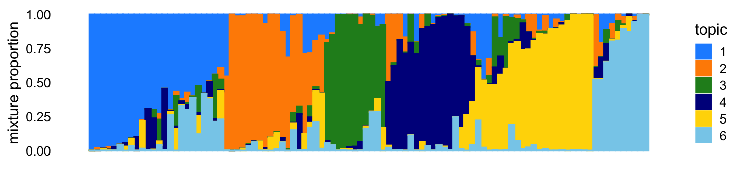
Here we compare two different updates for fitting a Poisson NMF model to the simulated counts: EM updates, and sequential coordinate descent (SCD). We perform 100 iterations of each. The model fitting is initialized by first running 50 EM updates, with the aim of better ensuring that the same local maximum is recovered by both runs.
control <- list(extrapolate = FALSE,numiter = 4)
fit0 <- fit_poisson_nmf(X,k,numiter = 50,method = "em",control = control)
fit1 <- fit_poisson_nmf(X,fit0=fit0,numiter=100,method="em",control=control)
fit2 <- fit_poisson_nmf(X,fit0=fit0,numiter=100,method="scd",control=control)
fit0 <- poisson2multinom(fit0)
fit1 <- poisson2multinom(fit1)
fit2 <- poisson2multinom(fit2)
This next plot shows the improvement in the solution over time for the EM and SCD updates. The Y axis shows the difference between the current log-likelihood and the best log-likelihood achieved by the two methods.
pdat <- rbind(data.frame(iter   = 1:150,
                         loglik = fit1$progress$loglik.multinom,
                         res    = fit1$progress$res,
                         method = "em"),
              data.frame(iter   = 1:150,
                         loglik = fit2$progress$loglik.multinom,
                         res    = fit2$progress$res,
                         method = "scd"))
pdat <- subset(pdat,iter >= 50)
pdat <- transform(pdat,
                  iter   = iter - 50,
                  loglik = max(loglik) - loglik + 0.1)
p2 <- ggplot(pdat,aes(x = iter,y = loglik,color = method)) +
  geom_line(size = 0.75) +
  scale_y_continuous(trans = "log10") +
  scale_color_manual(values = c("dodgerblue","darkorange")) +
  labs(x = "iteration",y = "loglik difference") +
  theme_cowplot(font_size = 10)
p3 <- ggplot(pdat,aes(x = iter,y = res,color = method)) +
  geom_line(size = 0.75) +
  scale_color_manual(values = c("dodgerblue","darkorange")) +
  labs(x = "iteration",y = "max KKT residual") +
  theme_cowplot(font_size = 10)
plot_grid(p2,p3)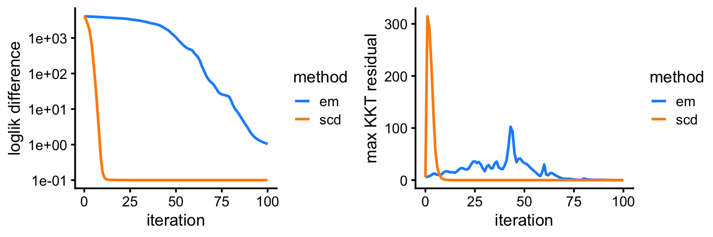
| Version | Author | Date |
|---|---|---|
| be1f9a4 | Peter Carbonetto | 2021-03-11 |
| daf189c | Peter Carbonetto | 2021-03-09 |
| 47ed425 | Peter Carbonetto | 2021-03-09 |
| 907addd | Peter Carbonetto | 2021-03-08 |
| 1838ec8 | Peter Carbonetto | 2021-03-08 |
| 50f34a9 | Peter Carbonetto | 2021-03-07 |
| 1185ab4 | Peter Carbonetto | 2021-03-07 |
| 913316c | Peter Carbonetto | 2021-03-07 |
| 51c5321 | Peter Carbonetto | 2021-03-06 |
| 59a8594 | Peter Carbonetto | 2021-03-05 |
| ffad471 | Peter Carbonetto | 2021-03-05 |
Among the two methods compared, the SCD updates progress more rapidly toward a solution. Still, the EM updates recover the same solution after a reasonable number of iterations. Indeed, the EM and SCD estimates of the topic proportions are almost the same:
p4 <- loadings_scatterplot(fit1,fit2,topic_colors,"em","scd")
print(p4)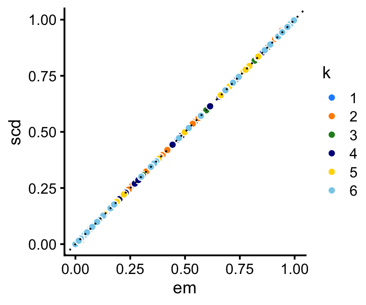
Add text here.
maptpx0 <- maptpx::topics(X,k,shape = 1,initopics = fit0$F,omega = fit0$L,
                          tol = 0.001,tmax = 1000,ord = FALSE,verb = 0)
maptpx1 <- maptpx::topics(X,k,shape = 1,initopics = fit1$F,omega = fit1$L,
                          tol = 0.001,tmax = 1000,ord = FALSE,verb = 0)
maptpx2 <- maptpx::topics(X,k,shape = 1,initopics = fit2$F,omega = fit2$L,
                          tol = 0.001,tmax = 1000,ord = FALSE,verb = 0)
Add text here.
pdat <- rbind(data.frame(iter = 1:length(maptpx0$progress),
                         y    = maptpx0$progress,
                         init = "em-50"),
              data.frame(iter = 1:length(maptpx1$progress),
                         y    = maptpx1$progress,
                         init = "em-150"),
              data.frame(iter = 1:length(maptpx2$progress),
                         y    = maptpx2$progress,
                         init = "scd"))
pdat <- transform(pdat,y = max(y) - y + 0.1)
ggplot(pdat,aes(x = iter,y = y,color = init)) +
  geom_line(size = 0.75) +
  scale_y_continuous(trans = "log10") +
  scale_color_manual(values = c("dodgerblue","darkblue","darkorange")) +
  labs(x = "iteration",y = "log-posterior difference") +
  theme_cowplot(font_size = 10)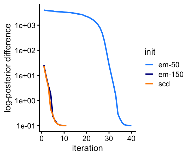
Next, we turn to the problem of fitting an LDA model to the same data.
We perform 400 iterations of variational EM, initializing the LDA model fits using the MLEs computed above.
lda0 <- run_lda(X,fit0,numiter = 400)
lda1 <- run_lda(X,fit1,numiter = 400)
lda2 <- run_lda(X,fit2,numiter = 400)
Warning: The above code chunk cached its results, but it won’t be re-run if previous chunks it depends on are updated. If you need to use caching, it is highly recommended to also set knitr::opts_chunk$set(autodep = TRUE) at the top of the file (in a chunk that is not cached). Alternatively, you can customize the option dependson for each individual chunk that is cached. Using either autodep or dependson will remove this warning. See the knitr cache options for more details.
Although the LDA fitting problem is different—we are now fitting a (approximate) posterior distribution, and so the estimates are approximate posterior means rather than MLE—initializing the LDA fit using the MLEs greatly improves the LDA model fitting, as we will see from this next plot: even after 400 iterations, variational EM without a good initialization does not approach the quality of the LDA model fits initialized using the EM and SCD estimates.
pdat <- rbind(data.frame(iter = 1:400,elbo = lda0@logLiks,init = "none"),
              data.frame(iter = 1:400,elbo = lda1@logLiks,init = "em"),
              data.frame(iter = 1:400,elbo = lda2@logLiks,init = "scd"))
pdat <- transform(pdat,elbo = max(elbo) - elbo + 0.1)
p5<-ggplot(pdat,aes(x = iter,y = elbo,color = init)) +
           geom_line(size = 0.75) +
           scale_y_continuous(trans = "log10") +
           scale_color_manual(values=c("darkblue","dodgerblue","darkorange")) +
           labs(x = "iteration",y = "ELBO difference") +
           theme_cowplot(font_size = 10)
print(p5)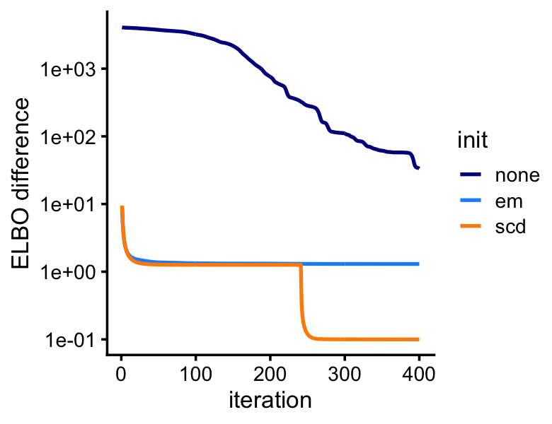
Next we will see an example in which EM updates fail to make reasonable progress.
Correlated topics scenario
The count data in this second example are simulated as before, with one difference: by setting \(s_{56} = s_{65} = 8\), the mixture proportions for topics 5 and 6 are no longer close to orthogonal.
set.seed(1)
S[5,6] <- 8
S[6,5] <- 8
L <- simulate_loadings(n,k,S)
X <- simulate_multinom_counts(L,F,s)
X <- X[,colSums(X > 0) > 0]
Compare this Structure plot to the one above—there is more mixing of topics 5 and 6:
p6 <- simdata_structure_plot(L,topic_colors)
print(p6)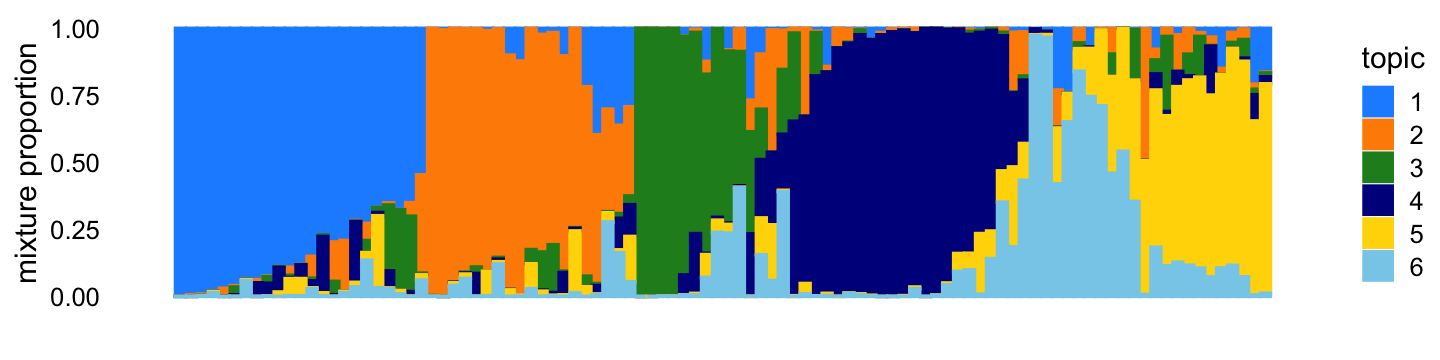
As before, we run the EM and SCD updates to fit the multinomial topic model, with a twist that we perform another round of SCD updates after running the EM updates. This will be explained shortly.
fit0 <- fit_poisson_nmf(X,k,numiter = 50,method = "em",control = control)
fit1 <- fit_poisson_nmf(X,fit0=fit0,numiter=750,method="em",control=control)
fit2 <- fit_poisson_nmf(X,fit0=fit0,numiter=950,method="scd",control=control)
fit3 <- fit_poisson_nmf(X,fit0=fit1,numiter=200,method="scd",control=control)
fit1 <- fit_poisson_nmf(X,fit0=fit1,numiter=200,method="em",control=control)
fit0 <- poisson2multinom(fit0)
fit1 <- poisson2multinom(fit1)
fit2 <- poisson2multinom(fit2)
fit3 <- poisson2multinom(fit3)
In this second example, after initially making good progress, the EM estimates remain far from the solution achieved by SCD even after hundreds of EM updates. This isn’t a case where the EM updates have settled on a different local solution—the SCD updates quickly “rescue” the EM estimates.
pdat <- rbind(data.frame(iter   = 1:1000,
                         loglik = fit1$progress$loglik.multinom,
                         res    = fit1$progress$res,
                         method = "em"),
              data.frame(iter   = 1:1000,
                         loglik = fit2$progress$loglik.multinom,
                         res    = fit2$progress$res,
                         method = "scd"),
              data.frame(iter   = 800:1000,
                         loglik = fit3$progress[800:1000,"loglik.multinom"],
                         res    = fit3$progress[800:1000,"res"],
                         method = "em+scd"))
pdat <- subset(pdat,iter >= 50)
pdat <- transform(pdat,
                  iter   = iter - 50,
                  loglik = max(loglik) - loglik + 0.1)
p7 <- ggplot(pdat,aes(x = iter,y = loglik,color = method)) +
  geom_line(size = 0.75) +
  scale_y_continuous(trans = "log10") +
  scale_color_manual(values = c("dodgerblue","darkorange","magenta")) +
  labs(x = "iteration",y = "loglik difference") +
  theme_cowplot(font_size = 10)
p8 <- ggplot(pdat,aes(x = iter,y = res,color = method)) +
  geom_line(size = 0.75) +
  scale_color_manual(values = c("dodgerblue","darkorange","magenta")) +
  ylim(0,10) +
  labs(x = "iteration",y = "max KKT residual") +
  theme_cowplot(font_size = 10)
plot_grid(p7,p8)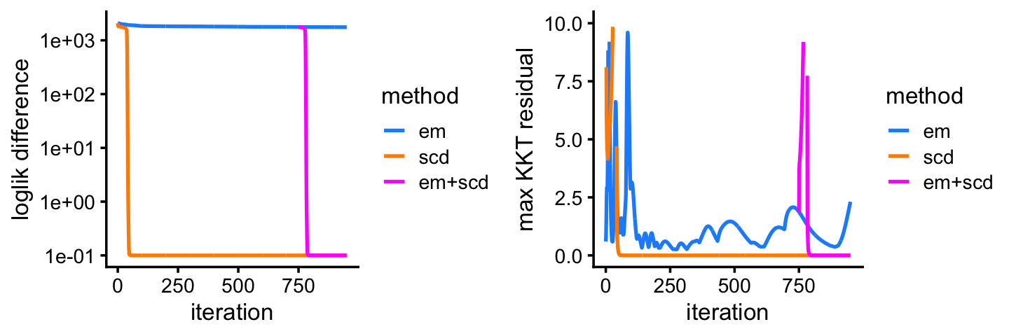
| Version | Author | Date |
|---|---|---|
| 311659c | Peter Carbonetto | 2021-03-12 |
| daf189c | Peter Carbonetto | 2021-03-09 |
| 47ed425 | Peter Carbonetto | 2021-03-09 |
| a967f97 | Peter Carbonetto | 2021-03-08 |
| 1838ec8 | Peter Carbonetto | 2021-03-08 |
| 50f34a9 | Peter Carbonetto | 2021-03-07 |
| 1185ab4 | Peter Carbonetto | 2021-03-07 |
| 7e3d55b | Peter Carbonetto | 2021-03-07 |
| 913316c | Peter Carbonetto | 2021-03-07 |
| 59a8594 | Peter Carbonetto | 2021-03-05 |
| ffad471 | Peter Carbonetto | 2021-03-05 |
This large difference in likelihood is not due to a trivial difference in solution—for example, there are many large differences in the topic proportion estimates:
p9 <- loadings_scatterplot(fit1,fit2,topic_colors,"em","scd")
print(p9)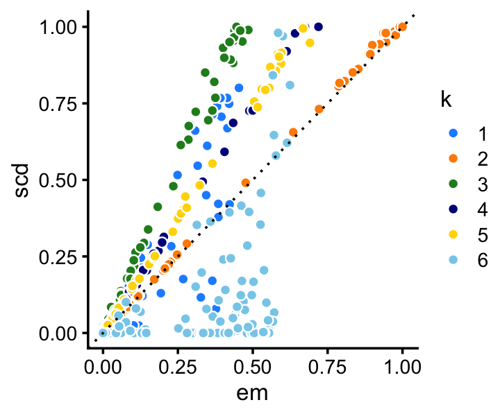
Most of the samples contributing to the large difference in likehood are samples generated from combinations of topics 5 and 6 (the X and Y axes in this scatterplot show the per-sample log-likelihoods):
pdat <- data.frame(x = loglik_multinom_topic_model(X,fit1),
                   y = loglik_multinom_topic_model(X,fit2))
ggplot(pdat,aes(x = x,y = y,fill = L[,5] + L[,6])) +
  geom_point(color = "white",shape = 21,size = 1.75) +
  geom_abline(intercept = 0,slope = 1,color = "black",linetype = "dotted") +
  scale_fill_gradient(low = "skyblue",high = "orangered") +
  xlim(-700,-100) +
  ylim(-700,-100) +
  labs(x = "em",y = "scd",fill = "topic 5 + 6") +
  theme_cowplot(font_size = 10)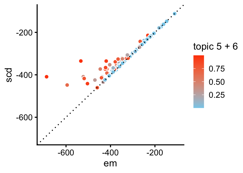
These results suggest that the EM algorithm may perform poorly in settings where the topics are correlated, even if the correlations are modest.
Let’s see how this relates to fitting an LDA model:
lda0 <- run_lda(X,fit0,numiter = 400)
lda1 <- run_lda(X,fit1,numiter = 400)
lda2 <- run_lda(X,fit2,numiter = 400)
Warning: The above code chunk cached its results, but it won’t be re-run if previous chunks it depends on are updated. If you need to use caching, it is highly recommended to also set knitr::opts_chunk$set(autodep = TRUE) at the top of the file (in a chunk that is not cached). Alternatively, you can customize the option dependson for each individual chunk that is cached. Using either autodep or dependson will remove this warning. See the knitr cache options for more details.
This plot shows the improvement in the objective (the ELBO) over time:
pdat <- rbind(data.frame(iter = 1:400,elbo = lda0@logLiks,init = "none"),
              data.frame(iter = 1:400,elbo = lda1@logLiks,init = "em"),
              data.frame(iter = 1:400,elbo = lda2@logLiks,init = "scd"))
pdat <- transform(pdat,elbo = max(elbo) - elbo + 0.1)
p10<-ggplot(pdat,aes(x = iter,y = elbo,color = init)) +
            geom_line(size = 0.75) +
            scale_y_continuous(trans = "log10") +
            scale_color_manual(values=c("darkblue","dodgerblue","darkorange"))+
            labs(x = "iteration",y = "ELBO difference") +
            theme_cowplot(font_size = 10)
print(p10)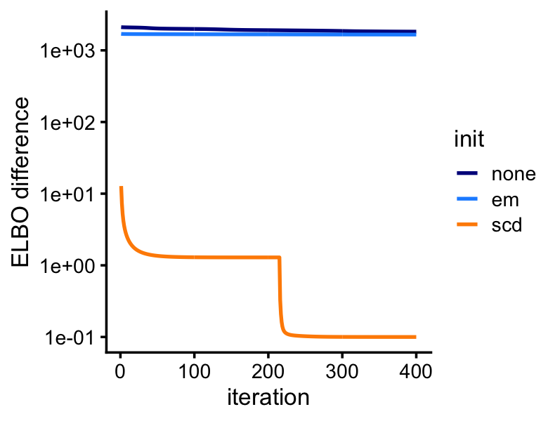
| Version | Author | Date |
|---|---|---|
| 311659c | Peter Carbonetto | 2021-03-12 |
In this second example, the SCD estimates provide by far the best initialization of the LDA model fit.
sessionInfo()
# R version 3.6.2 (2019-12-12)
# Platform: x86_64-apple-darwin15.6.0 (64-bit)
# Running under: macOS Catalina 10.15.7
#
# Matrix products: default
# BLAS:   /Library/Frameworks/R.framework/Versions/3.6/Resources/lib/libRblas.0.dylib
# LAPACK: /Library/Frameworks/R.framework/Versions/3.6/Resources/lib/libRlapack.dylib
#
# locale:
# [1] en_US.UTF-8/en_US.UTF-8/en_US.UTF-8/C/en_US.UTF-8/en_US.UTF-8
#
# attached base packages:
# [1] stats     graphics  grDevices utils     datasets  methods   base
#
# other attached packages:
# [1] cowplot_1.0.0     ggplot2_3.3.0     mvtnorm_1.0-11    fastTopics_0.5-24
# [5] topicmodels_0.2-9 tm_0.7-7          NLP_0.2-0
#
# loaded via a namespace (and not attached):
#  [1] httr_1.4.2           tidyr_1.0.0          jsonlite_1.6
#  [4] viridisLite_0.3.0    RcppParallel_4.4.2   assertthat_0.2.1
#  [7] mixsqp_0.3-44        stats4_3.6.2         progress_1.2.2
# [10] yaml_2.2.0           slam_0.1-47          ggrepel_0.9.0
# [13] pillar_1.4.3         backports_1.1.5      lattice_0.20-38
# [16] quadprog_1.5-8       quantreg_5.54        glue_1.3.1
# [19] digest_0.6.23        promises_1.1.0       colorspace_1.4-1
# [22] htmltools_0.4.0      httpuv_1.5.2         Matrix_1.3-3
# [25] pkgconfig_2.0.3      invgamma_1.1         SparseM_1.78
# [28] purrr_0.3.3          scales_1.1.0         whisker_0.4
# [31] later_1.0.0          Rtsne_0.15           MatrixModels_0.4-1
# [34] git2r_0.26.1         tibble_2.1.3         farver_2.0.1
# [37] withr_2.1.2          ashr_2.2-51          lazyeval_0.2.2
# [40] magrittr_1.5         crayon_1.3.4         mcmc_0.9-6
# [43] evaluate_0.14        fs_1.3.1             MASS_7.3-51.4
# [46] xml2_1.3.2           truncnorm_1.0-8      prettyunits_1.1.1
# [49] tools_3.6.2          data.table_1.12.8    hms_0.5.2
# [52] lifecycle_0.1.0      stringr_1.4.0        MCMCpack_1.4-5
# [55] plotly_4.9.2         munsell_0.5.0        irlba_2.3.3
# [58] compiler_3.6.2       rlang_0.4.5          grid_3.6.2
# [61] htmlwidgets_1.5.1    labeling_0.3         rmarkdown_2.3
# [64] codetools_0.2-16     gtable_0.3.0         R6_2.4.1
# [67] knitr_1.26           dplyr_0.8.3          zeallot_0.1.0
# [70] workflowr_1.6.2.9000 rprojroot_1.3-2      maptpx_1.9-8
# [73] modeltools_0.2-22    stringi_1.4.3        parallel_3.6.2
# [76] SQUAREM_2017.10-1    Rcpp_1.0.5           vctrs_0.2.1
# [79] tidyselect_0.2.5     xfun_0.11            coda_0.19-3