A closer look at some results on the newsgroups data
Peter Carbonetto
Last updated: 2024-08-08
Checks: 7 0
Knit directory:
fastTopics-experiments/analysis/
This reproducible R Markdown analysis was created with workflowr (version 1.7.1). The Checks tab describes the reproducibility checks that were applied when the results were created. The Past versions tab lists the development history.
Great! Since the R Markdown file has been committed to the Git repository, you know the exact version of the code that produced these results.
Great job! The global environment was empty. Objects defined in the global environment can affect the analysis in your R Markdown file in unknown ways. For reproduciblity it’s best to always run the code in an empty environment.
The command set.seed(1) was run prior to running the
code in the R Markdown file. Setting a seed ensures that any results
that rely on randomness, e.g. subsampling or permutations, are
reproducible.
Great job! Recording the operating system, R version, and package versions is critical for reproducibility.
Nice! There were no cached chunks for this analysis, so you can be confident that you successfully produced the results during this run.
Great job! Using relative paths to the files within your workflowr project makes it easier to run your code on other machines.
Great! You are using Git for version control. Tracking code development and connecting the code version to the results is critical for reproducibility.
The results in this page were generated with repository version 4c90df6. See the Past versions tab to see a history of the changes made to the R Markdown and HTML files.
Note that you need to be careful to ensure that all relevant files for
the analysis have been committed to Git prior to generating the results
(you can use wflow_publish or
wflow_git_commit). workflowr only checks the R Markdown
file, but you know if there are other scripts or data files that it
depends on. Below is the status of the Git repository when the results
were generated:
Ignored files:
    Ignored:    analysis/.sos/
    Ignored:    data/20news-bydate/
    Ignored:    data/droplet.RData
    Ignored:    data/nips_1-17.mat
    Ignored:    data/pbmc_68k.RData
    Ignored:    output/droplet/fits-droplet.RData
    Ignored:    output/droplet/lda-droplet.RData
    Ignored:    output/newsgroups/de-newsgroups.RData
    Ignored:    output/newsgroups/fits-newsgroups.RData
    Ignored:    output/newsgroups/lda-newsgroups.RData
    Ignored:    output/newsgroups/rds/
    Ignored:    output/nips/fits-nips.RData
    Ignored:    output/nips/lda-nips.RData
    Ignored:    output/pbmc68k/fits-pbmc68k.RData
    Ignored:    output/pbmc68k/rds/

Untracked files:
    Untracked:  analysis/lda-eb-newsgroups-em-k=10.rds
    Untracked:  analysis/lda-eb-newsgroups-scd-ex-k=10.rds
    Untracked:  analysis/lda-newsgroups-em-k=10.rds
    Untracked:  analysis/lda-newsgroups-scd-ex-k=10.rds
    Untracked:  analysis/maptpx-newsgroups-em-k=10.rds
    Untracked:  analysis/maptpx-newsgroups-scd-ex-k=10.rds
    Untracked:  plots/
Note that any generated files, e.g. HTML, png, CSS, etc., are not included in this status report because it is ok for generated content to have uncommitted changes.
These are the previous versions of the repository in which changes were
made to the R Markdown (analysis/newsgroups_more.Rmd) and
HTML (docs/newsgroups_more.html) files. If you’ve
configured a remote Git repository (see ?wflow_git_remote),
click on the hyperlinks in the table below to view the files as they
were in that past version.
| File | Version | Author | Date | Message |
|---|---|---|---|---|
| Rmd | 4c90df6 | Peter Carbonetto | 2024-08-08 | workflowr::wflow_publish("newsgroups_more.Rmd", verbose = TRUE) |
| Rmd | 7969f43 | Peter Carbonetto | 2024-08-07 | Working on new ‘newsgroups_more’ analysis. |
| html | a72103c | Peter Carbonetto | 2024-08-07 | First build of the newsgroups_more analysis. |
| Rmd | 269b84d | Peter Carbonetto | 2024-08-07 | workflowr::wflow_publish("newsgroups_more.Rmd") |
Here we take a closer look at some of the results on the newsgroups data.
Load the packages used in this analysis.
library(Matrix)
library(fastTopics)
library(ggplot2)
library(cowplot)
set.seed(1)
Load the newsgroups data.
load("../data/newsgroups.RData")Load the topic models fit using the EM and CD algorithms
fit1 <- readRDS("../output/newsgroups/rds/fit-newsgroups-em-k=10.rds")$fit
fit2 <- readRDS("../output/newsgroups/rds/fit-newsgroups-scd-ex-k=10.rds")$fit
fit1 <- poisson2multinom(fit1)
fit2 <- poisson2multinom(fit2)
and the LDA fits initialized using the EM and CD estimates:
lda1 <- readRDS("../output/newsgroups/rds/lda-newsgroups-em-k=10.rds")$lda
lda2 <- readRDS("../output/newsgroups/rds/lda-newsgroups-scd-ex-k=10.rds")$lda
The MLEs and the approximate posterior estimates from LDA turn out to be very similar to each other, so there is really no need to examine both. Here we’ll focus on the LDA fits:
cor(as.vector(fit1$L),as.vector(lda1@gamma))
cor(as.vector(fit2$L),as.vector(lda2@gamma))
# [1] 0.9799571
# [1] 0.9790959
Let’s now examine the LDA fits using Structure plots. Here is the EM-initialized model:
n <- nrow(fit1$L)
rows <- sample(n,2000)
L1 <- lda1@gamma[rows,]
topics <- factor(topics,
                 c("rec.sport.hockey",
                   "rec.sport.baseball",
                   "sci.med",
                   "comp.graphics",
                   "comp.windows.x",
                   "comp.os.ms-windows.misc",
                   "comp.sys.ibm.pc.hardware",
                   "comp.sys.mac.hardware",
                   "misc.forsale",
                   "sci.electronics",
                   "sci.space",
                   "alt.atheism",
                   "soc.religion.christian",
                   "talk.religion.misc",
                   "rec.autos",
                   "rec.motorcycles",
                   "sci.crypt",
                   "talk.politics.misc",
                   "talk.politics.guns",
                   "talk.politics.mideast"))
topic_ordering <- c(2:10,1)
topic_colors <- c("#a6cee3","#1f78b4","#b2df8a","#33a02c","#fb9a99",
                  "#e31a1c","#fdbf6f","#ff7f00","#cab2d6","#6a3d9a")
p1 <- structure_plot(L1,topics = 1:10,grouping = topics[rows],
                     colors = topic_colors,gap = 20) +
  ggtitle("EM without extrapolation") +
  theme(plot.title = element_text(face = "plain",size = 10))
p1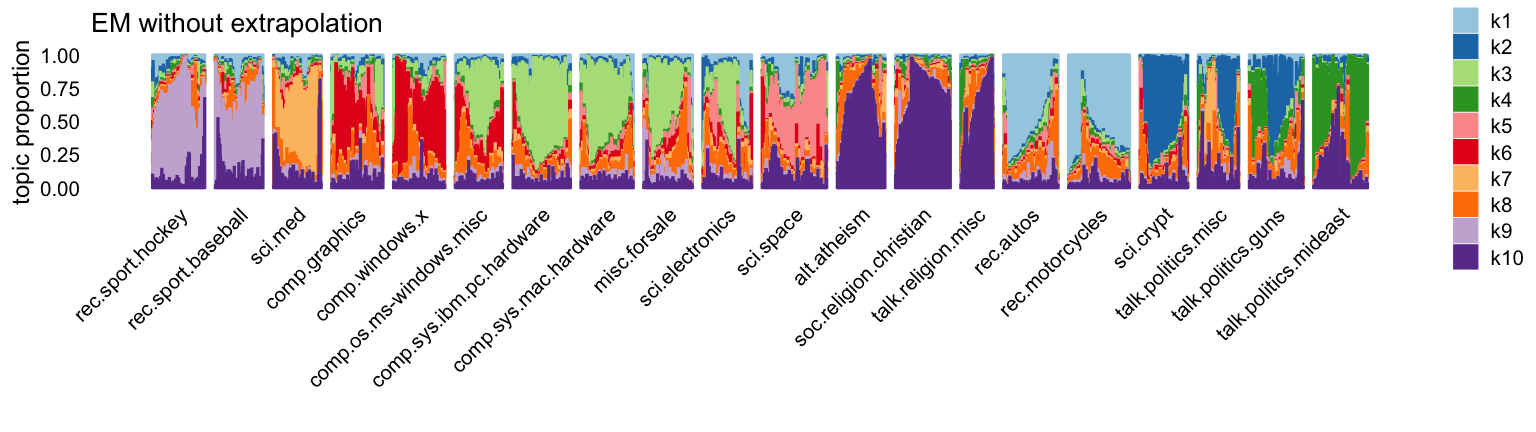
And here’s the CD-initialized model:
L2 <- lda2@gamma[rows,]
p2 <- structure_plot(L2,topics = 1:10,grouping = topics[rows],
                     colors = topic_colors,gap = 20) +
  ggtitle("CD with extrapolation") +
  theme(plot.title = element_text(face = "plain",size = 10))
p2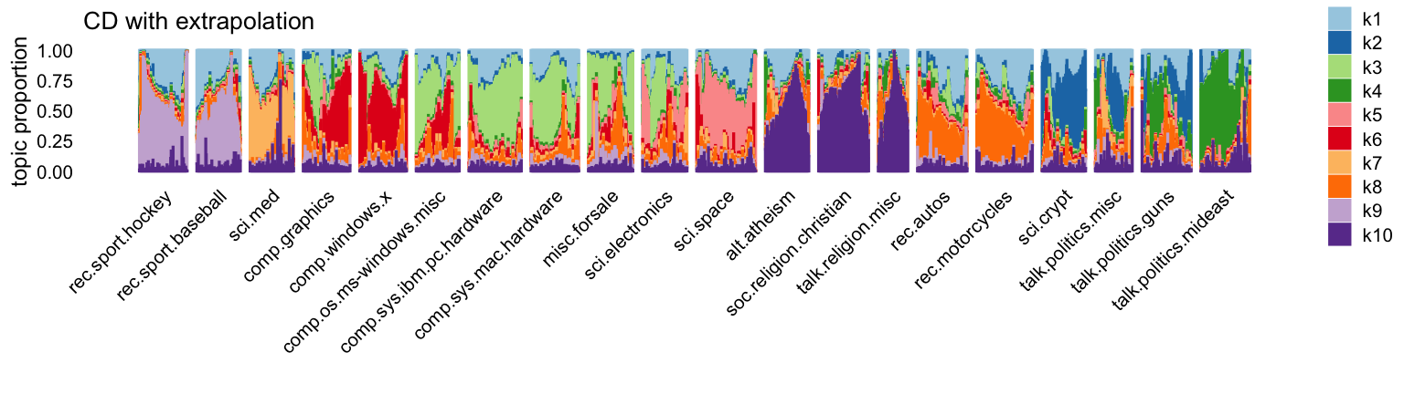
The most striking differences are in topics 1 and 8.
Let’s now extract some “keywords” for a few selected topics by taking words that are at higher frequency in the given topic compared to the other topics. For example, top keywords for topic 9 clearly relate to baseball, hockey and sports more generally:
k <- 9
dat <- data.frame(word = colnames(counts),
                  f0 = exp(apply(lda2@beta[-k,],2,max)),
                  f1 = exp(lda1@beta[k,]),
                  f2 = exp(lda2@beta[k,]))
subset(dat,f0 < 1e-5 & f2 > 1e-3)
#           word           f0           f1          f2
# 1815  baseball 2.810213e-26 0.0021858183 0.002558474
# 4306     teams 7.536962e-06 0.0014993384 0.001774011
# 7885       bos 1.246793e-74 0.0008952049 0.001047827
# 10219  players 7.288976e-09 0.0026286758 0.003076825
# 11252     fans 9.865409e-06 0.0015366619 0.001798602
# 26023   hockey 4.148975e-84 0.0028469414 0.003332311
# 26700      det 1.551769e-37 0.0009774498 0.001144093
# 26976  rangers 9.068849e-10 0.0009268376 0.001084851
# 27471  detroit 8.827394e-28 0.0010660214 0.001247765
# 32140     espn 9.498411e-85 0.0009489805 0.001110770
# 33823      nhl 6.136341e-96 0.0013412257 0.001569889
The keywords for topic 1 seem to suggest a “background topic” that captures words that are not specific to any topic:
k <- 1
dat <- data.frame(word = colnames(counts),
                  f0 = exp(apply(lda2@beta[-k,],2,max)),
                  f1 = exp(lda1@beta[k,]),
                  f2 = exp(lda2@beta[k,]))
subset(dat,f0 > 1e-6 & f2/f0 > 5)
#            word           f0           f1           f2
# 482        sure 2.730490e-04 1.318745e-03 2.004453e-03
# 826        just 1.104558e-03 5.767521e-03 6.867431e-03
# 849       keeps 1.961181e-05 8.763595e-05 1.180887e-04
# 861         don 5.529651e-04 5.307603e-03 8.014937e-03
# 964    anything 3.229690e-04 1.166993e-03 1.667917e-03
# 1089    happens 5.230439e-05 2.730698e-04 3.664144e-04
# 1101     wouldn 6.308532e-05 6.959523e-04 8.960805e-04
# 1114        isn 1.972071e-04 8.741999e-04 1.220989e-03
# 1122      going 2.382043e-04 1.970294e-03 2.556936e-03
# 1194      doesn 3.761664e-04 1.107042e-03 1.897569e-03
# 1243     really 2.449082e-04 2.363712e-03 2.940275e-03
# 1247    shouldn 4.291797e-05 1.892965e-04 3.218838e-04
# 1343      doing 2.023907e-04 7.380913e-04 1.175773e-03
# 1408      thing 3.595447e-04 1.748767e-03 1.818889e-03
# 1485      maybe 1.340824e-04 1.142698e-03 1.410303e-03
# 1542      guess 1.235434e-04 6.294977e-04 9.066628e-04
# 1702      worse 3.962225e-05 2.558826e-04 3.919230e-04
# 1943       glad 2.335043e-05 1.191823e-04 1.503062e-04
# 2380        lot 2.851634e-04 1.214309e-03 1.541849e-03
# 2511   complain 9.458426e-06 1.175283e-04 1.060635e-04
# 2625       aren 7.708783e-05 4.339988e-04 6.015582e-04
# 2936    wasting 1.146139e-05 5.363071e-05 5.774432e-05
# 3643   bothered 7.647129e-06 3.171709e-05 6.446484e-05
# 4728   homework 2.154784e-06 1.071034e-05 1.376657e-05
# 6772      scary 9.308367e-06 4.636186e-05 5.272061e-05
# 7946  obnoxious 3.811318e-06 1.502948e-05 2.142934e-05
# 9386   squashed 1.336997e-06 9.301078e-06 7.420718e-06
# 11847  figuring 6.026327e-06 2.689538e-05 3.307360e-05
# 14900 enjoyable 1.284264e-06 5.932311e-06 6.961532e-06
# 34566   ranting 2.708701e-06 4.813397e-22 1.498063e-05
# 49753   gloster 1.088760e-06 1.966287e-25 5.751089e-06
Finally, topic 8 is a topic that is quite noticeably different between the EM and CD estimates, and indeed based on the keywords, only the CD estimates produce a topic about cars and motorcycles, with keywords such as wheel, riding, bmw, etc:
k <- 8
dat <- data.frame(word = colnames(counts),
                  f0 = exp(apply(lda2@beta[-k,],2,max)),
                  f1 = exp(lda1@beta[k,]),
                  f2 = exp(lda2@beta[k,]))
subset(dat,f0 < 1e-5 & f2 > 5e-4)
#              word            f0           f1           f2
# 6685        wheel  2.926216e-06 2.574153e-48 0.0008890773
# 8379       riding  4.806729e-06 8.342523e-50 0.0010296821
# 8848          bmw  1.420484e-70 8.974584e-35 0.0014199092
# 10461     mustang  1.001845e-62 1.474671e-54 0.0005334919
# 10632        ford  6.054076e-09 9.614501e-05 0.0012188125
# 11034      helmet  7.566853e-06 6.205450e-57 0.0007346685
# 11456          di  6.241188e-07 7.696027e-04 0.0006960997
# 13843         mov 1.530331e-112 6.423834e-04 0.0005786335
# 14968          cx  1.896083e-06 5.944685e-04 0.0005342605
# 17351          ei  9.225139e-79 7.107221e-04 0.0006401903
# 18581        bike  4.785774e-57 1.148546e-61 0.0034348671
# 25666  motorcycle  6.819658e-06 4.778873e-48 0.0009843613
# 25691      toyota  6.852661e-34 1.203084e-46 0.0005293881
# 25947       honda  1.179594e-74 1.174884e-22 0.0009602854
# 26114       brake  4.286054e-06 5.328490e-92 0.0006481378
# 26116       tires  4.017934e-06 3.018378e-61 0.0007099675
# 27848       bikes  2.086974e-59 1.708530e-51 0.0008084454
# 27947 motorcycles  1.105482e-56 9.860881e-45 0.0005663222
sessionInfo()
# R version 4.3.3 (2024-02-29)
# Platform: aarch64-apple-darwin20 (64-bit)
# Running under: macOS Sonoma 14.5
#
# Matrix products: default
# BLAS:   /Library/Frameworks/R.framework/Versions/4.3-arm64/Resources/lib/libRblas.0.dylib
# LAPACK: /Library/Frameworks/R.framework/Versions/4.3-arm64/Resources/lib/libRlapack.dylib;  LAPACK version 3.11.0
#
# locale:
# [1] en_US.UTF-8/en_US.UTF-8/en_US.UTF-8/C/en_US.UTF-8/en_US.UTF-8
#
# time zone: America/Chicago
# tzcode source: internal
#
# attached base packages:
# [1] stats     graphics  grDevices utils     datasets  methods   base
#
# other attached packages:
# [1] cowplot_1.1.3      ggplot2_3.5.0      fastTopics_0.6-184 Matrix_1.6-5
#
# loaded via a namespace (and not attached):
#  [1] gtable_0.3.4        xfun_0.42           bslib_0.6.1
#  [4] htmlwidgets_1.6.4   ggrepel_0.9.5       lattice_0.22-5
#  [7] quadprog_1.5-8      vctrs_0.6.5         tools_4.3.3
# [10] generics_0.1.3      parallel_4.3.3      tibble_3.2.1
# [13] fansi_1.0.6         highr_0.10          pkgconfig_2.0.3
# [16] data.table_1.15.2   SQUAREM_2021.1      RcppParallel_5.1.7
# [19] lifecycle_1.0.4     truncnorm_1.0-9     farver_2.1.1
# [22] compiler_4.3.3      stringr_1.5.1       git2r_0.33.0
# [25] progress_1.2.3      munsell_0.5.0       RhpcBLASctl_0.23-42
# [28] httpuv_1.6.14       htmltools_0.5.7     sass_0.4.8
# [31] yaml_2.3.8          lazyeval_0.2.2      plotly_4.10.4
# [34] crayon_1.5.2        later_1.3.2         pillar_1.9.0
# [37] jquerylib_0.1.4     whisker_0.4.1       tidyr_1.3.1
# [40] uwot_0.1.16         cachem_1.0.8        gtools_3.9.5
# [43] tidyselect_1.2.1    digest_0.6.34       Rtsne_0.17
# [46] stringi_1.8.3       dplyr_1.1.4         purrr_1.0.2
# [49] ashr_2.2-66         labeling_0.4.3      rprojroot_2.0.4
# [52] fastmap_1.1.1       grid_4.3.3          colorspace_2.1-0
# [55] cli_3.6.2           invgamma_1.1        magrittr_2.0.3
# [58] utf8_1.2.4          withr_3.0.0         prettyunits_1.2.0
# [61] scales_1.3.0        promises_1.2.1      rmarkdown_2.26
# [64] httr_1.4.7          workflowr_1.7.1     hms_1.1.3
# [67] pbapply_1.7-2       evaluate_0.23       knitr_1.45
# [70] viridisLite_0.4.2   irlba_2.3.5.1       rlang_1.1.3
# [73] Rcpp_1.0.12         mixsqp_0.3-54       glue_1.7.0
# [76] jsonlite_1.8.8      R6_2.5.1            fs_1.6.3