UKBiobank Blood Cell

Last updated: 2020-10-27

Checks: 7 0

Knit directory: finemap-uk-biobank/

This reproducible R Markdown analysis was created with workflowr (version 1.6.1). The Checks tab describes the reproducibility checks that were applied when the results were created. The Past versions tab lists the development history.

R Markdown file: up-to-date

Great! Since the R Markdown file has been committed to the Git repository, you know the exact version of the code that produced these results.

Environment: empty

Great job! The global environment was empty. Objects defined in the global environment can affect the analysis in your R Markdown file in unknown ways. For reproduciblity it’s best to always run the code in an empty environment.

Seed: set.seed(20191114)

The command set.seed(20191114) was run prior to running the code in the R Markdown file. Setting a seed ensures that any results that rely on randomness, e.g. subsampling or permutations, are reproducible.

Session information: recorded

Great job! Recording the operating system, R version, and package versions is critical for reproducibility.

Cache: none

Nice! There were no cached chunks for this analysis, so you can be confident that you successfully produced the results during this run.

File paths: relative

Great job! Using relative paths to the files within your workflowr project makes it easier to run your code on other machines.

Repository version: d20e2e8

Great! You are using Git for version control. Tracking code development and connecting the code version to the results is critical for reproducibility.

The results in this page were generated with repository version d20e2e8. See the Past versions tab to see a history of the changes made to the R Markdown and HTML files.

Note that you need to be careful to ensure that all relevant files for the analysis have been committed to Git prior to generating the results (you can use wflow_publish or wflow_git_commit). workflowr only checks the R Markdown file, but you know if there are other scripts or data files that it depends on. Below is the status of the Git repository when the results were generated:


Ignored files:
    Ignored:    .DS_Store
    Ignored:    .Rhistory
    Ignored:    .Rproj.user/
    Ignored:    analysis/.Rhistory
    Ignored:    scripts/.DS_Store

Untracked files:
    Untracked:  data/bloodcounts.csv
    Untracked:  data/height.chr3.matrix
    Untracked:  data/susie_ss_input_sex.rds

Unstaged changes:
    Modified:   analysis/compare_result_more.Rmd

Note that any generated files, e.g. HTML, png, CSS, etc., are not included in this status report because it is ok for generated content to have uncommitted changes.

These are the previous versions of the repository in which changes were made to the R Markdown (analysis/bloodcells.Rmd) and HTML (docs/bloodcells.html) files. If you’ve configured a remote Git repository (see ?wflow_git_remote), click on the hyperlinks in the table below to view the files as they were in that past version.

File	Version	Author	Date	Message
Rmd	d20e2e8	zouyuxin	2020-10-27	wflow_publish(“analysis/bloodcells.Rmd”)

The UkB blood cell traits are

PheID	Abbrev	Phenotype	Cell type
30000	WBCcount	White blood cell count	Compound white cell
30010	RBCcount	Red blood cell count	Mature red cell
30020	HGB	Haemoglobin concentration	Mature red cell
30030	HCT	Haematocrit percentage	Mature red cell
30040	MCV	Mean corpuscular volume	Mature red cell
30050	MCH	Mean corpuscular haemoglobin	Mature red cell
30060	MCHC	Mean corpuscular haemoglobin concentration	Mature red cell
30070	RDW	Red blood cell distribution width	Mature red cell
30080	PLTcount	Platelet count	Platelet
30090	PCT	Platelet crit	Platelet
30100	MPV	Mean platelet (thrombocyte) volume	Platelet
30110	PDW	Platelet distribution width	Platelet
30120	LYMPHcount	Lymphocyte count	Lymphoid white cell
30130	MONOcount	Monocyte count	Myeloid white cell
30140	NEUTcount	Neutrophill count	Myeloid white cell
30150	EOcount	Eosinophill count	Myeloid white cell
30160	BASOcount	Basophill count	Myeloid white cell
30180	LYMPHperc	Lymphocyte percentage	Compound white cell
30190	MONOperc	Monocyte percentage	Compound white cell
30200	NEUTperc	Neutrophill percentage	Compound white cell
30210	EOperc	Eosinophill percentage	Compound white cell
30220	BASOperc	Basophill percentage	Compound white cell
30240	RETperc	Reticulocyte percentage	Immature red cell
30250	RETcount	Reticulocyte count	Immature red cell
30260	MRV	Mean reticulocyte volume	Immature red cell
30270	MSCV	Mean sphered cell volume	Mature red cell
30280	IRF	Immature reticulocyte fraction	Immature red cell
30290	HLRperc	High light scatter reticulocyte percentage	Immature red cell
30300	HLRcount	High light scatter reticulocyte count	Immature red cell

We filtered individuals with following criteria:

Remove samples with missing values.
Remove samples that are not marked as being “White British”.
Remove samples with mismatches between self-reported and genetic sex.
Remove outliers defined by UK Biobank.
Remove any individuals have at leat one relative based on the kinship calculations.
Remove any pregnant individuals.
Remove any individuals with following in hospital in-patient data:

leukemia, lymphoma, bone marrow transplant, chemotherapy, myelodysplastic syndrome, anemia, HIV, end-stage kidney disease, dialysis, cirrhosis, multiple myeloma, lymphocytic leukemia, myeloid leukemia, polycythaemia vera, haemochromatosis

Load UKBiobank Blood Cell traits (individuals are filtered using script)

library(data.table)
library(dplyr)
dat = fread('data/bloodcounts.csv')
class(dat) <- "data.frame"

There are 257604 individuals.

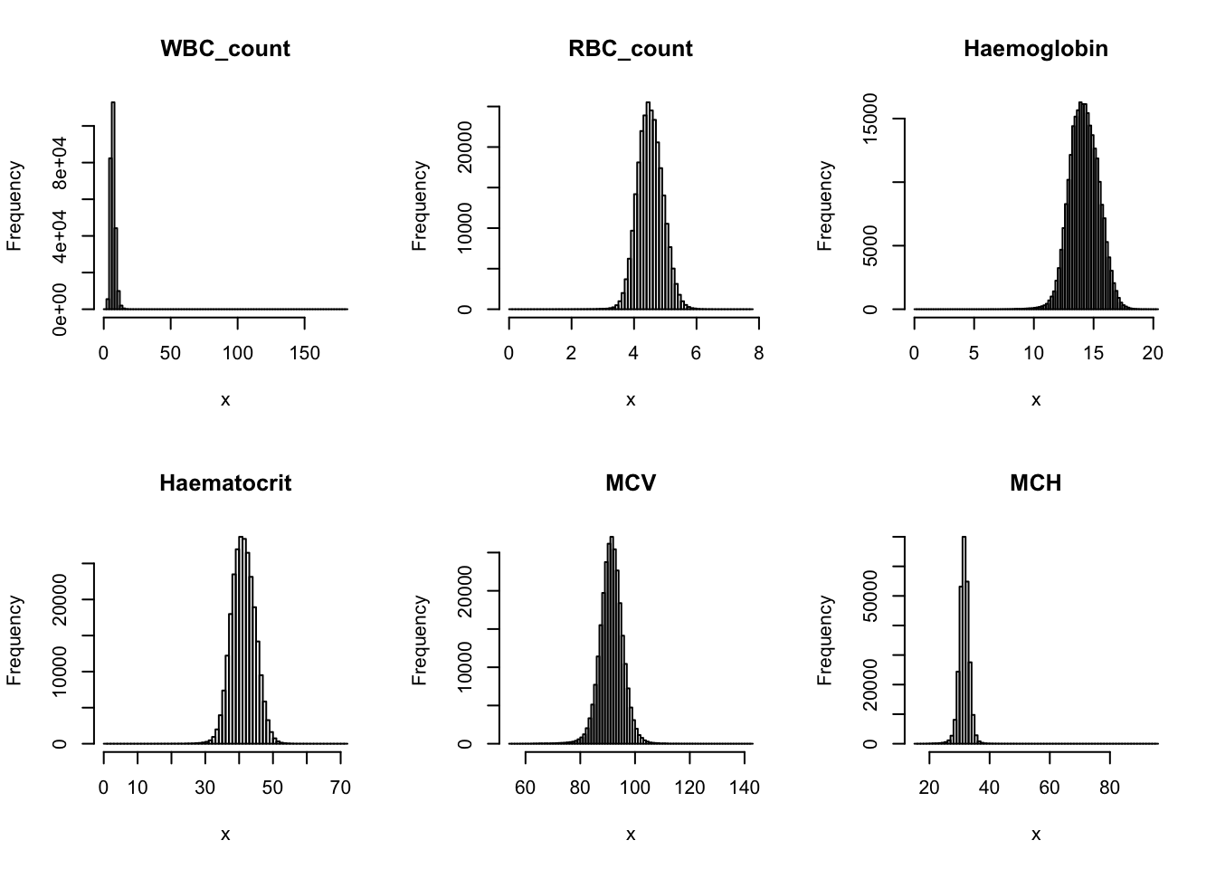
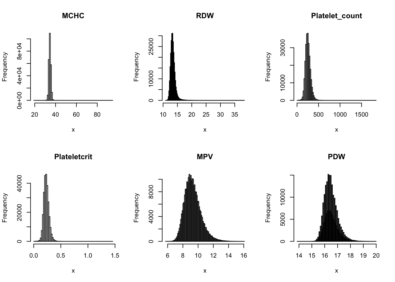
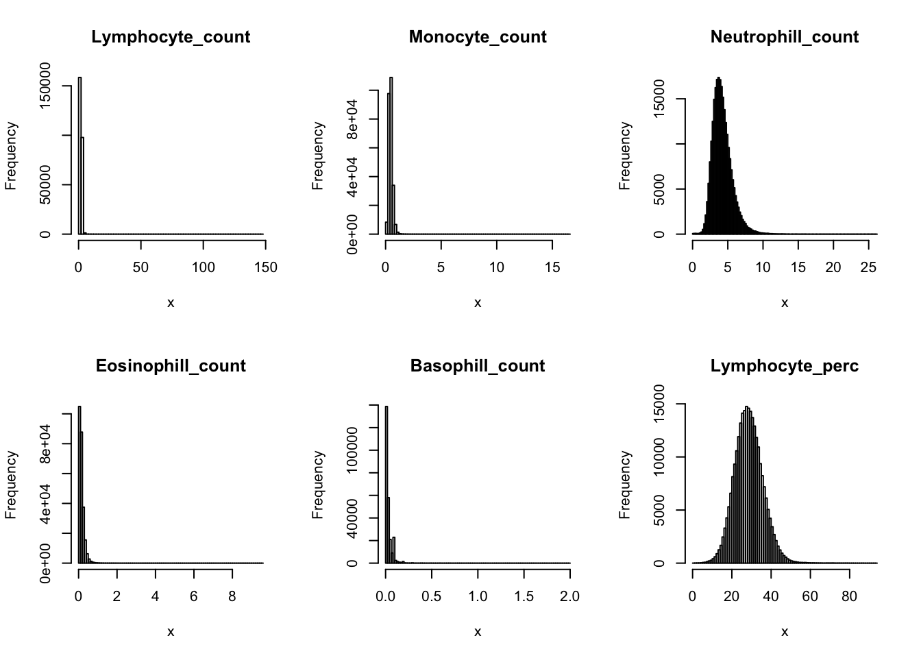
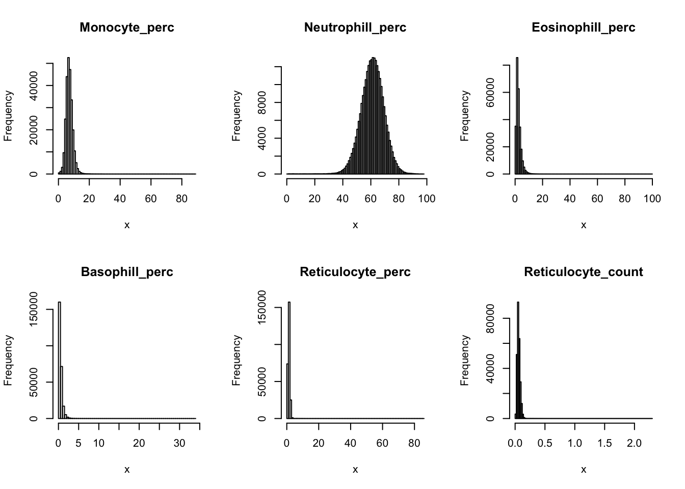
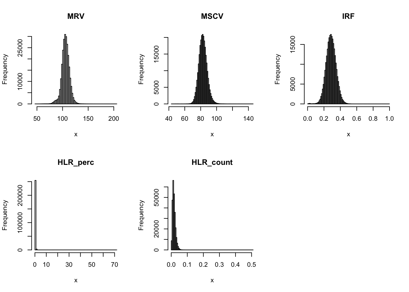
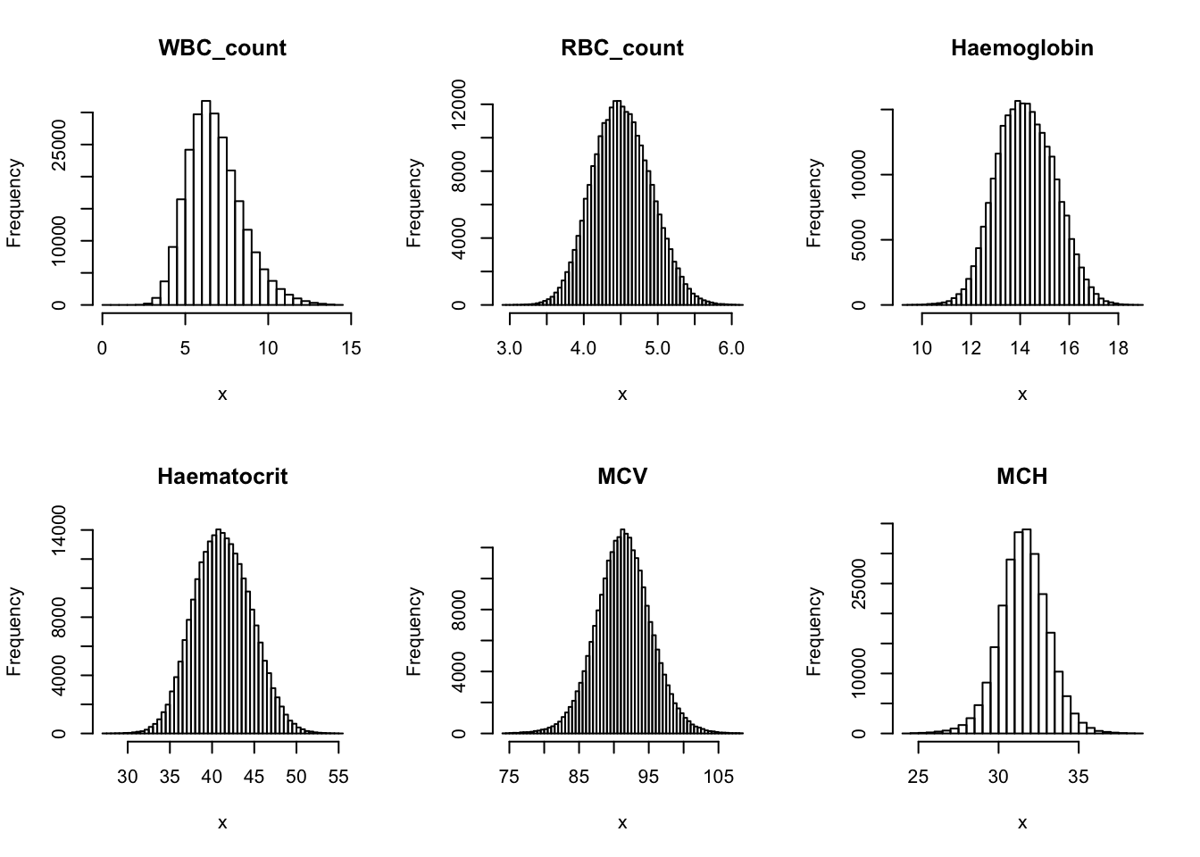
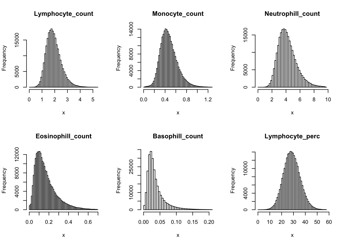
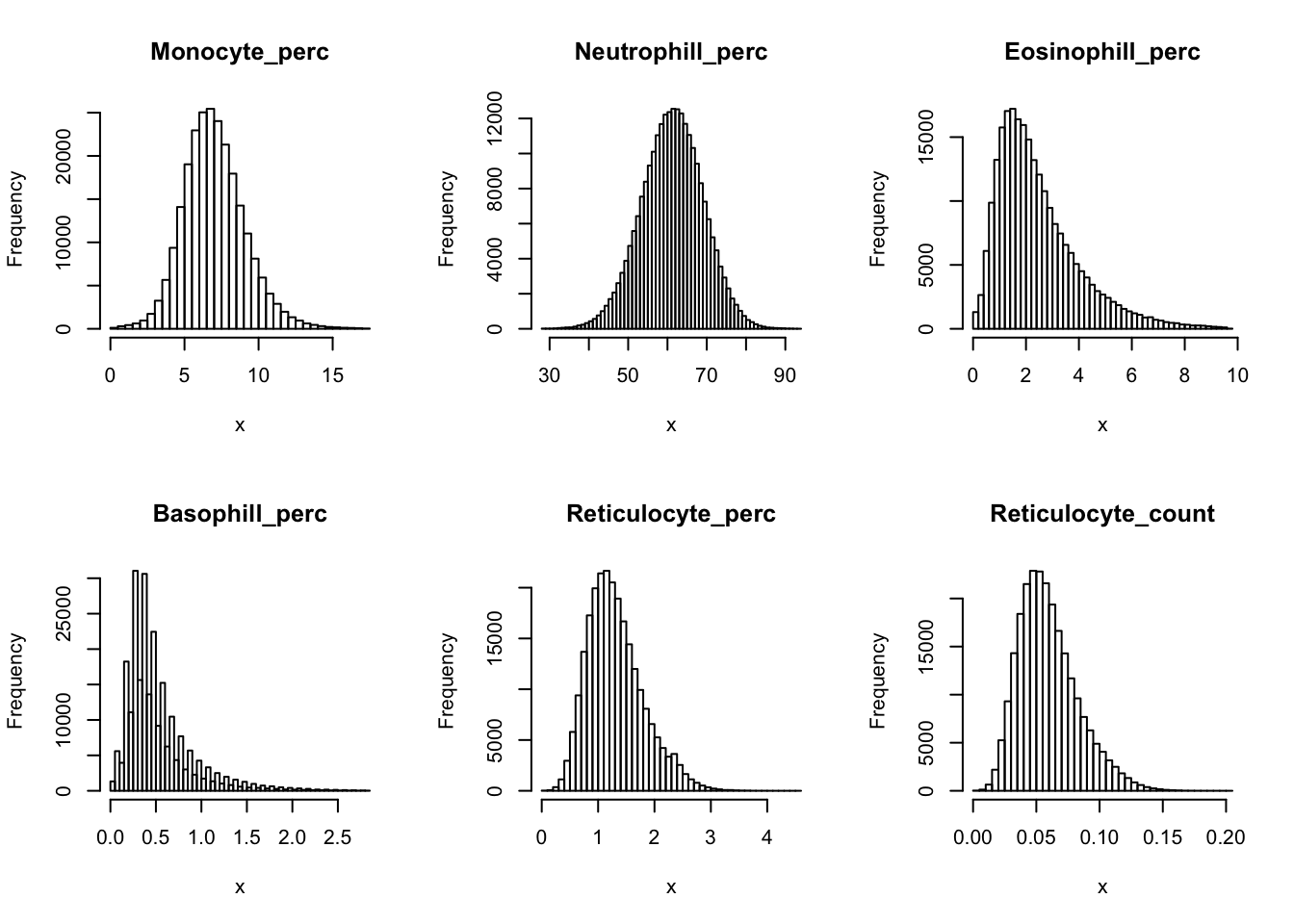
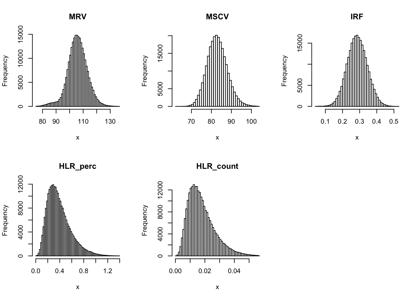
Check distribution for each trait:

par(mfrow=c(2,3))
for(i in 16:44){
  hist(dat[,i], breaks = 100, main=colnames(dat)[i], xlab='x')
}

Distributions for trait with small observartions:

par(mfrow=c(2,3))
hist(dat$WBC_count[dat$WBC_count < 20], breaks = 100, main=paste0('WBC_count ', sum(dat$WBC_count > 20), ' inds > 20'), xlab='x')
hist(dat$Lymphocyte_count[dat$Lymphocyte_count < 8], breaks = 100, main=paste0('Lymphocyte_count ', sum(dat$Lymphocyte_count > 8), ' inds > 8'), xlab='x')
hist(dat$Monocyte_count[dat$Monocyte_count < 2], breaks = 100, main=paste0('Monocyte_count ', sum(dat$Monocyte_count > 2), ' inds > 2'), xlab='x')
hist(dat$Eosinophill_count[dat$Eosinophill_count < 1], breaks = 100, main=paste0('Eosinophill_count ', sum(dat$Eosinophill_count > 1), ' inds > 1'), xlab='x')
hist(dat$Eosinophill_perc[dat$Eosinophill_perc < 10], breaks = 100, main=paste0('Eosinophill_perc ', sum(dat$Eosinophill_perc > 10), ' inds > 10'), xlab='x')
hist(dat$Basophill_count[dat$Basophill_count < 0.5], breaks = 100, main=paste0('Basophill_count ', sum(dat$Basophill_count > 0.5), ' inds > 0.5'), xlab='x')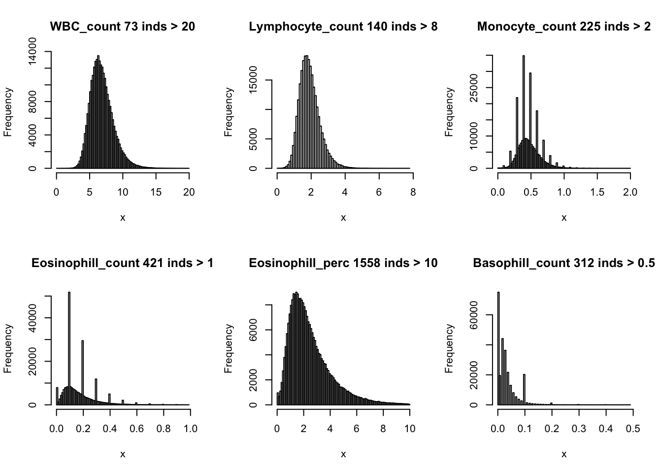

hist(dat$Basophill_perc[dat$Basophill_perc < 2], breaks = 100, main=paste0('Basophill_perc ', sum(dat$Basophill_perc > 2), ' inds > 2'), xlab='x')
hist(dat$Reticulocyte_count[dat$Reticulocyte_count < 0.2], breaks = 100, main=paste0('Reticulocyte_count ', sum(dat$Reticulocyte_count > 0.2), ' inds > 0.2'), xlab='x')
hist(dat$Reticulocyte_perc[dat$Reticulocyte_perc < 4], breaks = 100, main=paste0('Reticulocyte_perc ', sum(dat$Reticulocyte_perc > 4), ' inds > 4'), xlab='x')
hist(dat$HLR_count[dat$HLR_count < 0.1], breaks = 100, main=paste0('HLR_count ', sum(dat$HLR_count > 0.1), ' inds > 0.1'), xlab='x')
hist(dat$HLR_perc[dat$HLR_perc < 2], breaks = 100, main=paste0('HLR_perc ', sum(dat$HLR_perc > 2), ' inds > 2'), xlab='x')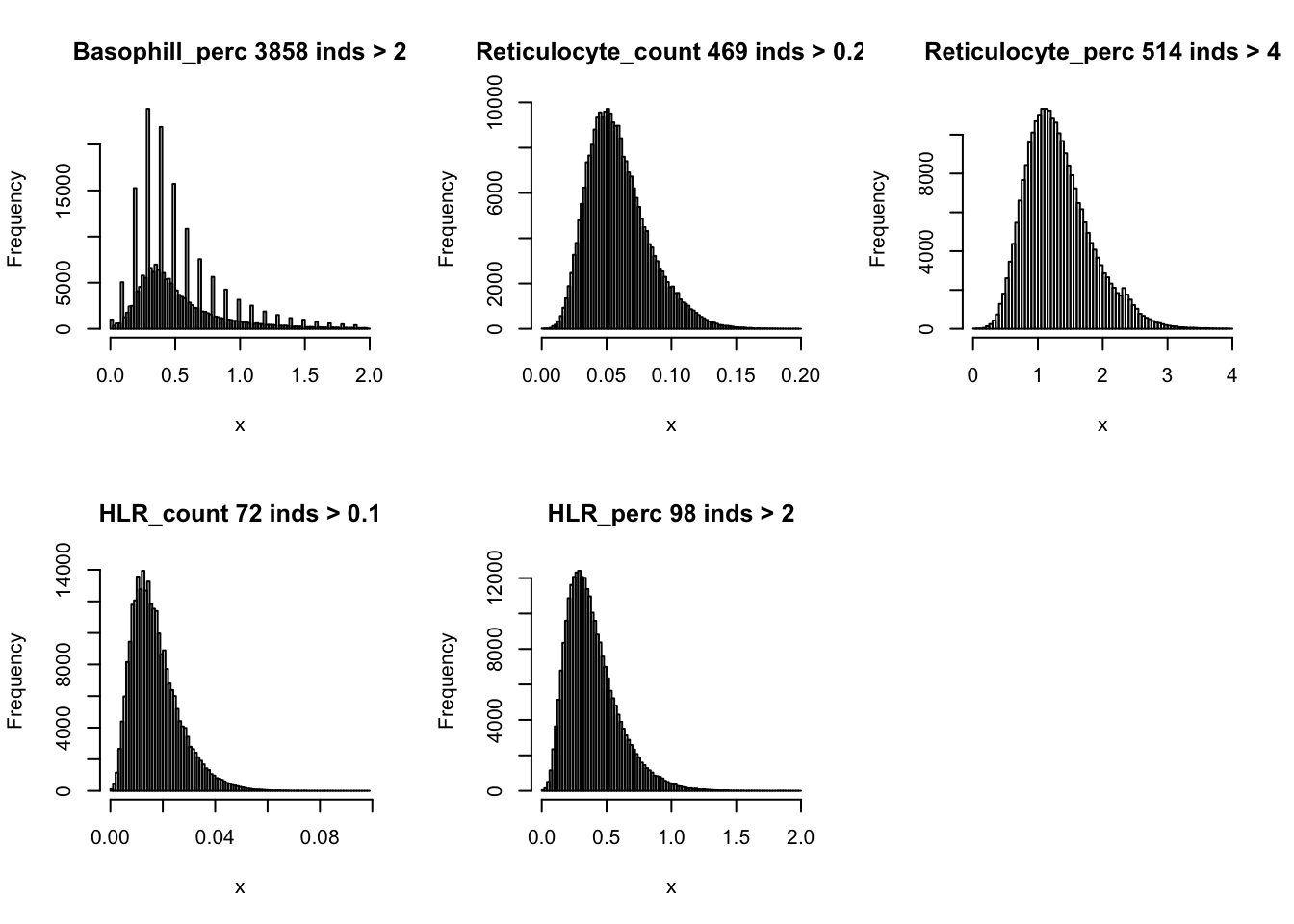

Basophill

Basophils count is the proportion of ( basophils / 100 ) x white blood cell count.

Basophils_count = dat$Basophill_perc * dat$WBC_count / 100
{plot(Basophils_count, dat$Basophill_count, ylab='UKB Basophill count')
abline(0,1)}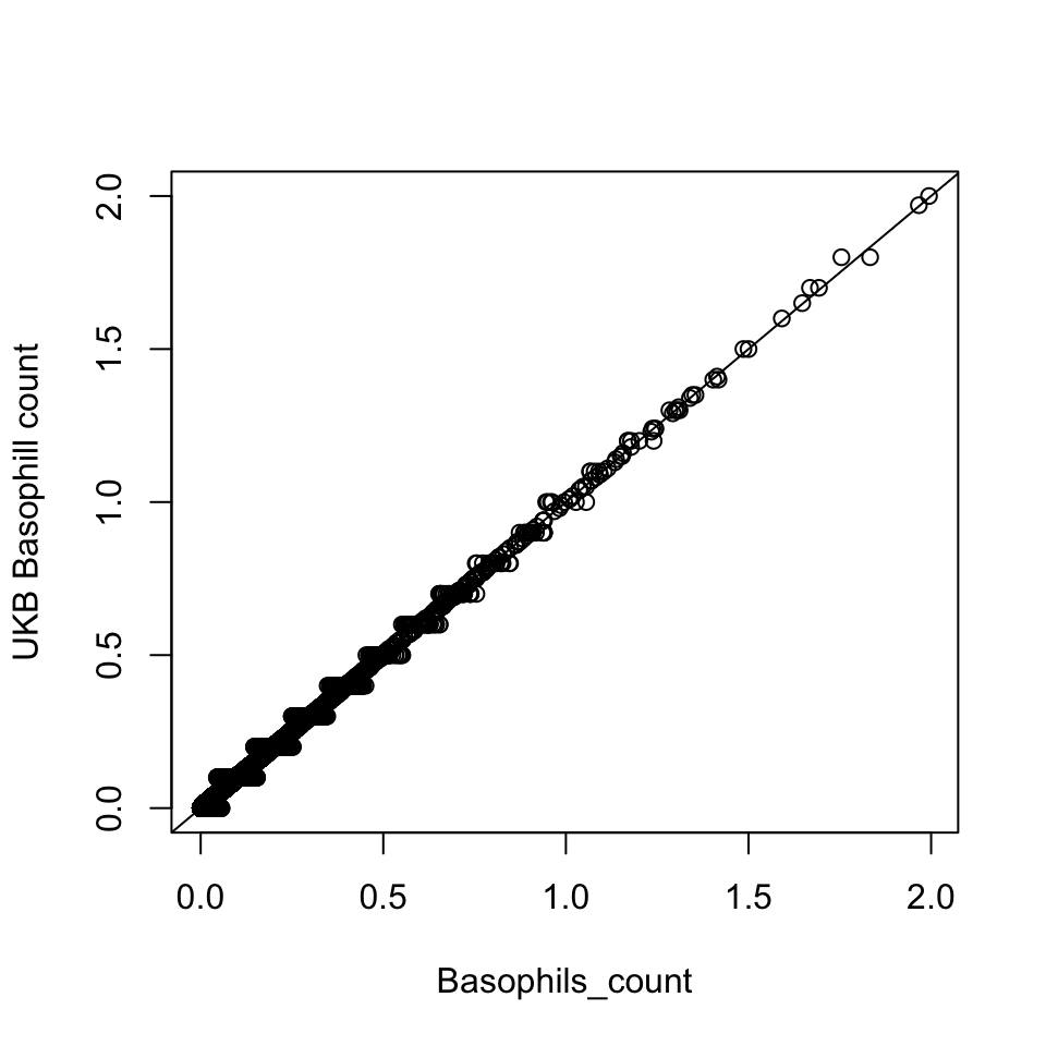

There are 835 0’s in computed Basophils_count, but there are 75056 0’s in UKB Basophils count.

hist(Basophils_count[Basophils_count < 0.5], breaks = 100, main=paste0('Derived Basophils_count ', sum(Basophils_count > 0.5), ' inds > 0.5'), xlab='x')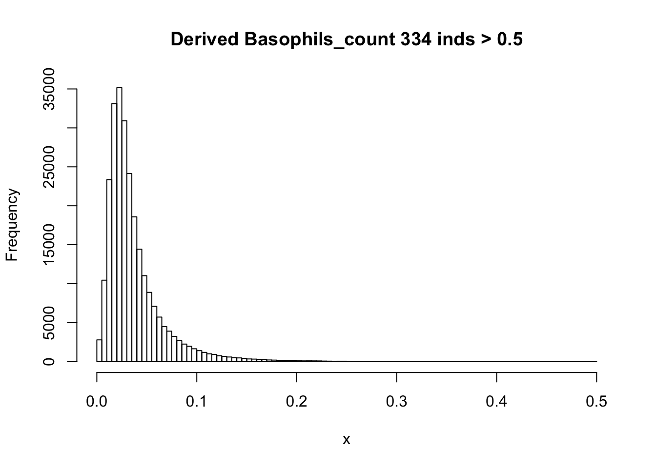

There are rounding errors in derived count traits.

We recompute all derived traits.

dat$Haematocrit = (dat$MCV * dat$RBC_count)/10
dat$MCH = (dat$Haemoglobin/dat$RBC_count) * 10
dat$MCHC = (dat$Haemoglobin/dat$Haematocrit)*100
dat$Lymphocyte_count = (dat$Lymphocyte_perc * dat$WBC_count)/100
dat$Monocyte_count = (dat$Monocyte_perc * dat$WBC_count)/100
dat$Eosinophill_count = (dat$Eosinophill_perc * dat$WBC_count)/100
dat$Basophill_count = (dat$Basophill_perc * dat$WBC_count)/100
dat$Reticulocyte_count = (dat$Reticulocyte_perc * dat$RBC_count)/100
dat$HLR_count = (dat$HLR_perc * dat$RBC_count)/100

par(mfrow=c(2,3))
hist(dat$WBC_count[dat$WBC_count < 20], breaks = 100, main=paste0('WBC_count ', sum(dat$WBC_count > 20), ' inds > 20'), xlab='x')
hist(dat$Lymphocyte_count[dat$Lymphocyte_count < 8], breaks = 100, main=paste0('Lymphocyte_count ', sum(dat$Lymphocyte_count > 8), ' inds > 8'), xlab='x')
hist(dat$Monocyte_count[dat$Monocyte_count < 2], breaks = 100, main=paste0('Monocyte_count ', sum(dat$Monocyte_count > 2), ' inds > 2'), xlab='x')
hist(dat$Eosinophill_count[dat$Eosinophill_count < 1], breaks = 100, main=paste0('Eosinophill_count ', sum(dat$Eosinophill_count > 1), ' inds > 1'), xlab='x')
hist(dat$Eosinophill_perc[dat$Eosinophill_perc < 10], breaks = 100, main=paste0('Eosinophill_perc ', sum(dat$Eosinophill_perc > 10), ' inds > 10'), xlab='x')
hist(dat$Basophill_count[dat$Basophill_count < 0.5], breaks = 100, main=paste0('Basophill_count ', sum(dat$Basophill_count > 0.5), ' inds > 0.5'), xlab='x')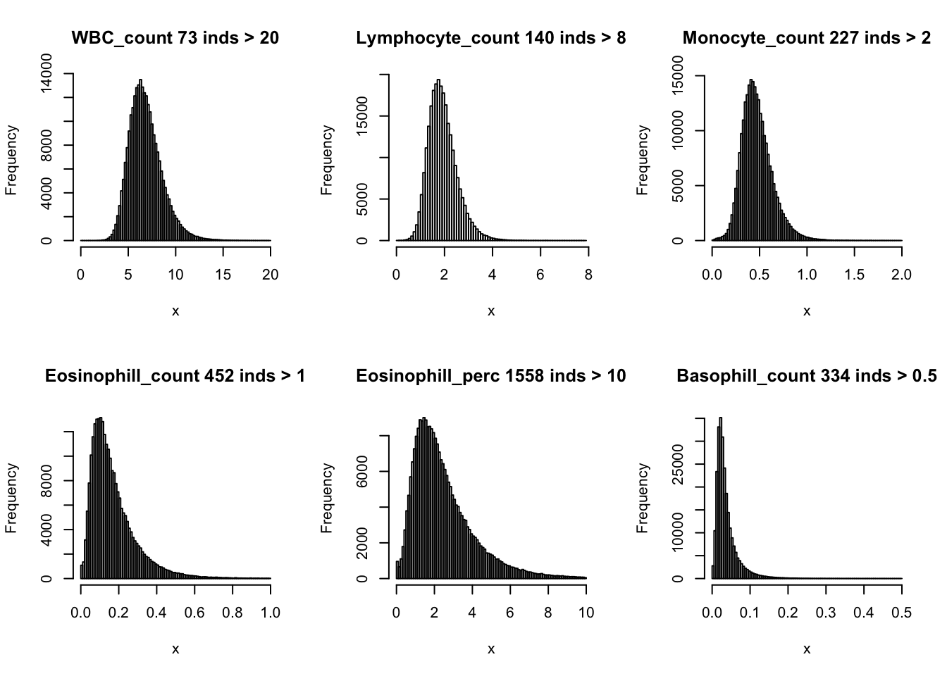

hist(dat$Basophill_perc[dat$Basophill_perc < 2], breaks = 100, main=paste0('Basophill_perc ', sum(dat$Basophill_perc > 2), ' inds > 2'), xlab='x')
hist(dat$Reticulocyte_count[dat$Reticulocyte_count < 0.2], breaks = 100, main=paste0('Reticulocyte_count ', sum(dat$Reticulocyte_count > 0.2), ' inds > 0.2'), xlab='x')
hist(dat$Reticulocyte_perc[dat$Reticulocyte_perc < 4], breaks = 100, main=paste0('Reticulocyte_perc ', sum(dat$Reticulocyte_perc > 4), ' inds > 4'), xlab='x')
hist(dat$HLR_count[dat$HLR_count < 0.1], breaks = 100, main=paste0('HLR_count ', sum(dat$HLR_count > 0.1), ' inds > 0.1'), xlab='x')
hist(dat$HLR_perc[dat$HLR_perc < 2], breaks = 100, main=paste0('HLR_perc ', sum(dat$HLR_perc > 2), ' inds > 2'), xlab='x')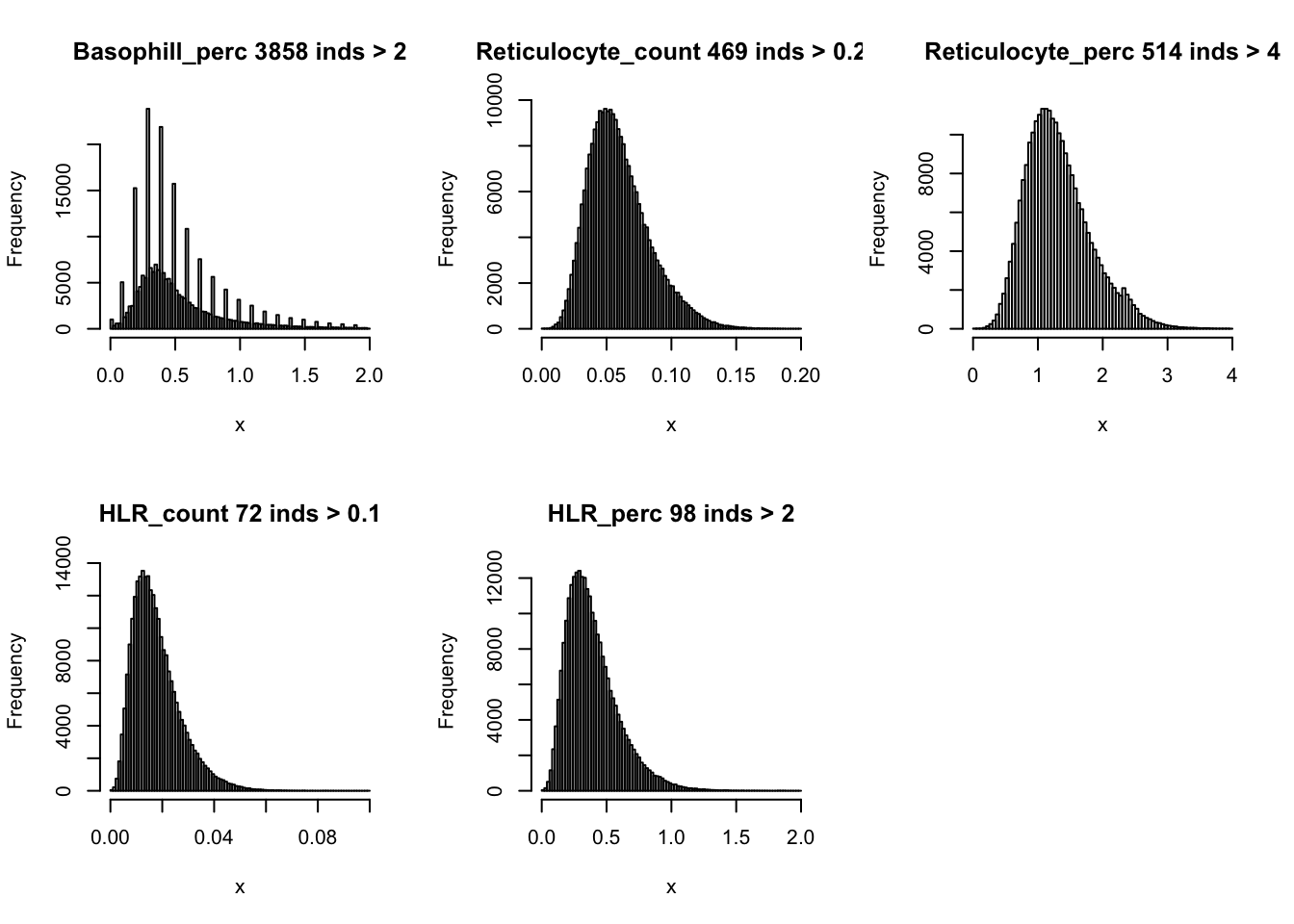

Remove extreme observatios

rem = c()
for(i in 16:44){
  rem = c(rem, which(dat[,i] < (median(dat[,i]) - 4*sqrt(mean((dat[,i] - median(dat[,i]))^2))) | dat[,i] > (median(dat[,i]) + 4*sqrt(mean((dat[,i] - median(dat[,i]))^2)))))
}
## remove 12758 individuals
dat_1 = dat[-unique(rem),]

par(mfrow=c(2,3))
for(i in 16:44){
  hist(dat_1[,i], breaks = 50, main=colnames(dat_1)[i], xlab='x')
}

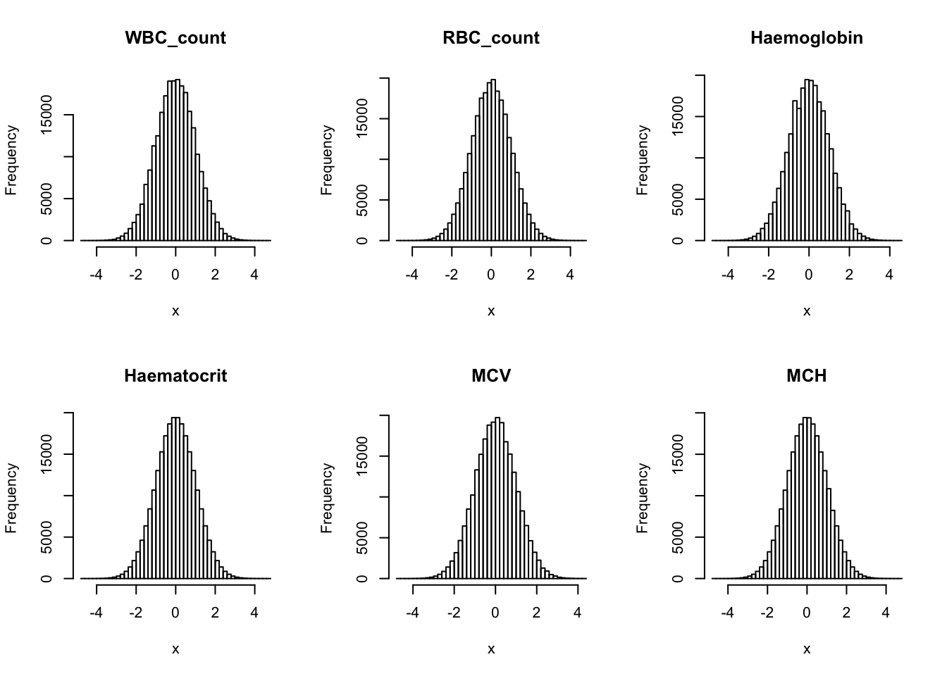
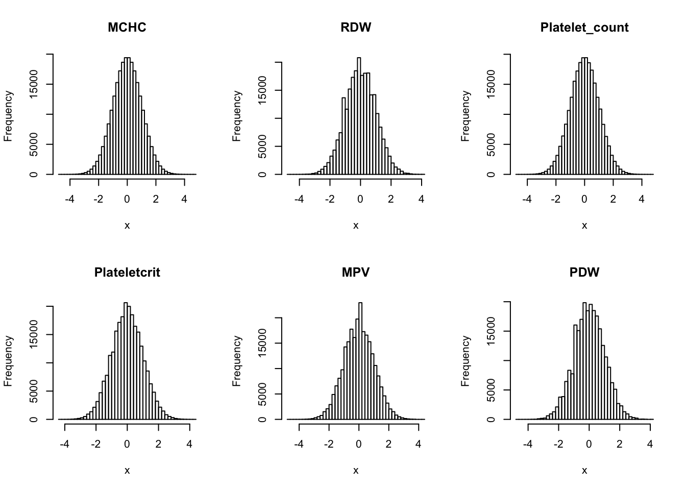
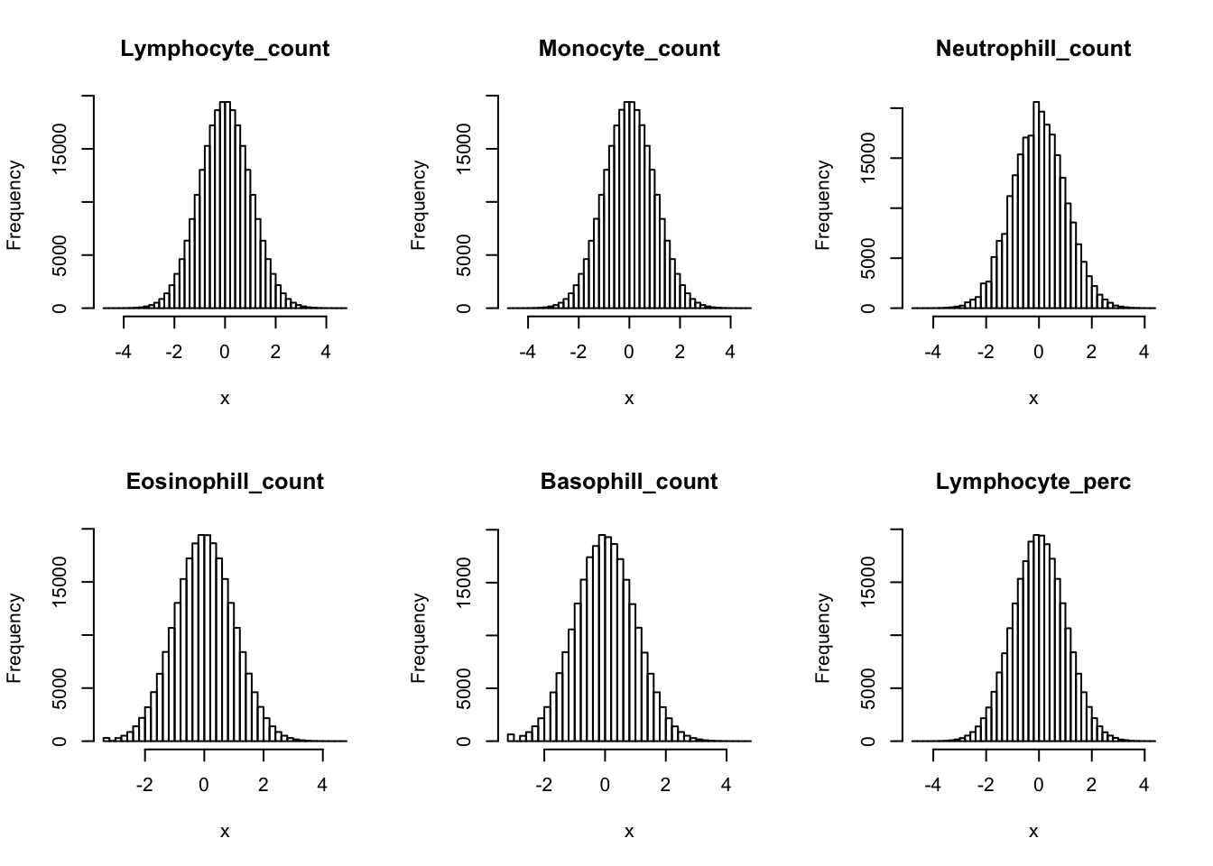
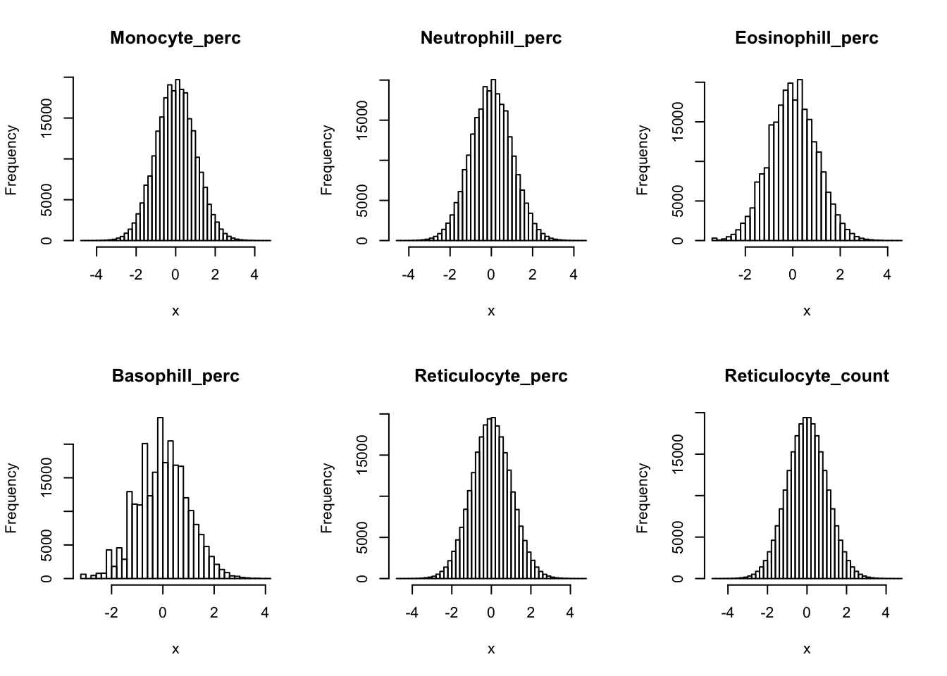
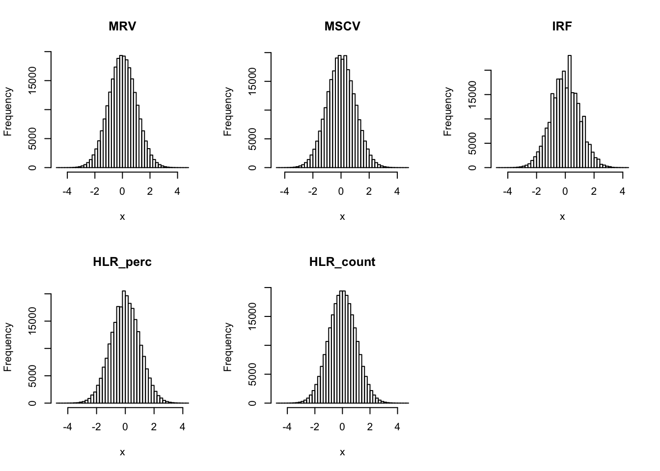
Inverse normalization:

dat_2 = dat_1
for(i in 16:44){
  dat_2[,i] = qnorm((rank(dat_2[,i],na.last="keep")-0.5)/sum(!is.na(dat_2[,i])))
}

par(mfrow=c(2,3))
for(i in 16:44){
  hist(dat_2[,i], breaks = 50, main=colnames(dat_2)[i], xlab='x')
}

sessionInfo()

R version 3.6.3 (2020-02-29)
Platform: x86_64-apple-darwin15.6.0 (64-bit)
Running under: macOS Catalina 10.15.7

Matrix products: default
BLAS:   /Library/Frameworks/R.framework/Versions/3.6/Resources/lib/libRblas.0.dylib
LAPACK: /Library/Frameworks/R.framework/Versions/3.6/Resources/lib/libRlapack.dylib

locale:
[1] en_US.UTF-8/en_US.UTF-8/en_US.UTF-8/C/en_US.UTF-8/en_US.UTF-8

attached base packages:
[1] stats     graphics  grDevices utils     datasets  methods   base     

other attached packages:
[1] dplyr_0.8.5       data.table_1.12.8 workflowr_1.6.1  

loaded via a namespace (and not attached):
 [1] Rcpp_1.0.5       knitr_1.28       whisker_0.4      magrittr_1.5    
 [5] tidyselect_1.0.0 R6_2.4.1.9001    rlang_0.4.8      stringr_1.4.0   
 [9] tools_3.6.3      xfun_0.13        git2r_0.26.1     ellipsis_0.3.1  
[13] htmltools_0.4.0  yaml_2.2.1       digest_0.6.27    rprojroot_1.3-2 
[17] assertthat_0.2.1 lifecycle_0.2.0  tibble_3.0.4     crayon_1.3.4    
[21] purrr_0.3.4      later_1.0.0      vctrs_0.3.4      promises_1.1.0  
[25] fs_1.4.1         glue_1.4.2       evaluate_0.14    rmarkdown_2.1   
[29] stringi_1.5.3    pillar_1.4.6     compiler_3.6.3   backports_1.1.10
[33] httpuv_1.5.2     pkgconfig_2.0.3

UKBiobank Blood Cell

Yuxin Zou

10/26/2020

Basophill