Fine-mapping Height ZBTB38 – SuSiE check
Yuxin Zou
10/07/2019
Last updated: 2019-11-19
Checks: 7 0
Knit directory: finemap-uk-biobank/
This reproducible R Markdown analysis was created with workflowr (version 1.5.0). The Checks tab describes the reproducibility checks that were applied when the results were created. The Past versions tab lists the development history.
Great! Since the R Markdown file has been committed to the Git repository, you know the exact version of the code that produced these results.
Great job! The global environment was empty. Objects defined in the global environment can affect the analysis in your R Markdown file in unknown ways. For reproduciblity it’s best to always run the code in an empty environment.
The command set.seed(20191114) was run prior to running the code in the R Markdown file. Setting a seed ensures that any results that rely on randomness, e.g. subsampling or permutations, are reproducible.
Great job! Recording the operating system, R version, and package versions is critical for reproducibility.
Nice! There were no cached chunks for this analysis, so you can be confident that you successfully produced the results during this run.
Great job! Using relative paths to the files within your workflowr project makes it easier to run your code on other machines.
Great! You are using Git for version control. Tracking code development and connecting the code version to the results is critical for reproducibility. The version displayed above was the version of the Git repository at the time these results were generated.
Note that you need to be careful to ensure that all relevant files for the analysis have been committed to Git prior to generating the results (you can use wflow_publish or wflow_git_commit). workflowr only checks the R Markdown file, but you know if there are other scripts or data files that it depends on. Below is the status of the Git repository when the results were generated:
Untracked files:
    Untracked:  data/height.ACAN.XtX.Xty.rds
    Untracked:  data/height.ADAMTS10.XtX.Xty.rds
    Untracked:  data/height.ADAMTS17.XtX.Xty.rds
    Untracked:  data/height.ADAMTSL3.XtX.Xty.rds
    Untracked:  data/height.CABLES1.XtX.Xty.rds
    Untracked:  data/height.CDK6.XtX.Xty.rds
    Untracked:  data/height.DLEU1.XtX.Xty.rds
    Untracked:  data/height.EFEMP1.XtX.Xty.rds
    Untracked:  data/height.GDF5.XtX.Xty.rds
    Untracked:  data/height.GNA12.XtX.Xty.rds
    Untracked:  data/height.HHIP.XtX.Xty.rds
    Untracked:  data/height.HMGA2.XtX.Xty.rds
    Untracked:  data/height.KDM2A.XtX.Xty.rds
    Untracked:  data/height.LCORL.XtX.Xty.rds
    Untracked:  data/height.MTMR11.XtX.Xty.rds
    Untracked:  data/height.UQCC1.XtX.Xty.rds
    Untracked:  data/height.ZBTB38.0.01.simulation1000.rds
    Untracked:  data/height.ZBTB38.XtX.Xty.rds
    Untracked:  data/height.ZBTB38.neale.rds
    Untracked:  data/height.ZBTB38.removeCS1.XtX.Xty.rds
    Untracked:  data/height.ZBTB38.removeCS2.XtX.Xty.rds
    Untracked:  data/height.ZBTB38.susie.model.rds
    Untracked:  output/height.CABLES1.removeCS1.XtX.Xty.rds
    Untracked:  output/height.CABLES1.removeCS2.XtX.Xty.rds
    Untracked:  output/height.GDF5.removeCS1.XtX.Xty.rds
    Untracked:  output/height.ZBTB38.plink2.height.glm.linear
    Untracked:  output/height.ZBTB38.removeCS1.XtX.Xty.rds
    Untracked:  output/height.ZBTB38.removeCS2.XtX.Xty.rds
    Untracked:  output/height.ZBTB38.simulation1000.rds
    Untracked:  output/height.ZBTB38.susie.model.rds

Unstaged changes:
    Modified:   analysis/_site.yml
    Modified:   analysis/finemap_height_CABLES1_check.Rmd
    Modified:   analysis/index.Rmd
    Modified:   scripts/plots.R
    Modified:   scripts/prepare.region.sh
    Modified:   scripts/prepare.susieinput.R
Note that any generated files, e.g. HTML, png, CSS, etc., are not included in this status report because it is ok for generated content to have uncommitted changes.
These are the previous versions of the R Markdown and HTML files. If you’ve configured a remote Git repository (see ?wflow_git_remote), click on the hyperlinks in the table below to view them.
| File | Version | Author | Date | Message |
|---|---|---|---|---|
| Rmd | f71bb43 | zouyuxin | 2019-11-20 | wflow_publish(“analysis/finemap_height_ZBTB38_check.Rmd”) |
| html | 149b7c7 | zouyuxin | 2019-11-19 | Build site. |
| Rmd | c14d255 | zouyuxin | 2019-11-19 | wflow_publish(“analysis/finemap_height_ZBTB38_check.Rmd”) |
| html | 9b47ac3 | zouyuxin | 2019-11-17 | move html files to docs |
| Rmd | 36beabb | zouyuxin | 2019-11-13 | update result with inputation score filtered data |
| Rmd | 4173d7a | zouyuxin | 2019-10-12 | update plot |
| Rmd | d6870cf | zouyuxin | 2019-10-12 | update plots |
| Rmd | 89a3e6c | zouyuxin | 2019-10-09 | change title; add detailed checks for 2 regions |
We perform some check for the SuSiE result on region around ZBTB38.
Load pacakges:
library(readr)
library(dplyr)
library(gridExtra)
library(susieR)
Load plotting functions:
knitr::read_chunk("scripts/plots.R")library(ggplot2)
#' plot gene name annotations
#' @param dat a matrix of gene names with 'start' and 'end' base-pair position
#' @param xrange range of x axis, base-pair position
plot_geneName = function(dat, xrange, chr){
ngene = 2:nrow(dat)
line = 1
dat$lines = NA
dat$lines[1] = 1
gene.end = dat[1, 'end']
while(length(ngene) != 0){
id = which(dat[ngene, 'start'] > gene.end + 0.02)[1]
if(!is.na(id)){
dat$lines[ngene[id]] = line
gene.end = dat[ngene[id],'end']
ngene = ngene[-id]
}else{
line = line + 1
dat$lines[ngene[1]] = line
gene.end = dat[ngene[1],'end']
ngene = ngene[-1]
}
}
dat$start = pmax(dat$start, xrange[1])
dat$end = pmin(dat$end, xrange[2])
dat$mean = rowMeans(dat[,c('start', 'end')])
pl = ggplot(dat, aes(xmin = xrange[1], xmax = xrange[2])) + xlim(xrange[1], xrange[2]) + ylim(min(-dat$lines-0.6), -0.8) +
geom_rect(aes(xmin = start, xmax = end, ymin = -lines-0.05, ymax = -lines+0.05), fill='blue') +
geom_text(aes(x = mean, y=-lines-0.4, label=geneName), size=4) +
xlab(paste0('base-pair position (Mb) on chromosome ', chr)) + ylab('Gene') +
theme_bw() + theme(axis.text.x=element_blank(),
axis.ticks = element_blank(),
axis.text.y=element_blank(),
axis.title = element_text(size=15),
plot.title=element_text(size=11),
panel.grid.major = element_blank(),
panel.grid.minor = element_blank())
pl
}
discrete_gradient_pal <- function(colours, bins = 5) {
ramp <- scales::colour_ramp(colours)
function(x) {
if (length(x) == 0) return(character())
i <- floor(x * bins)
i <- ifelse(i > bins-1, bins-1, i)
ramp(i/(bins-1))
}
}
scale_colour_discrete_gradient <- function(..., colours, bins = 5, na.value = "grey50", guide = "colourbar", aesthetics = "colour", colors) {
colours <- if (missing(colours))
colors
else colours
continuous_scale(
aesthetics,
"discrete_gradient",
discrete_gradient_pal(colours, bins),
na.value = na.value,
guide = guide,
...
)
}
#' Locuszoom plot
#' @param z a vector of z scores with SNP names
#' @param pos base-pair positions
#' @param gene.pos.map a matrix of gene names with 'start' and 'end' base-pair position
#' @param z.ref.name the reference SNP
#' @param ld correlations between teh reference SNP and the rests
#' @param title title of the plot
#' @param title.size the size of the title
#' @param true the true value
#' @param y.height height of -log10(p) plot and height of the gene name annotation plot
#' @param y.lim range of y axis
locus.zoom = function(z, pos, chr, gene.pos.map=NULL, z.ref.name=NULL, ld=NULL,
title = NULL, title.size = 10, true = NULL,
y.height=c(5,1.5), y.lim=NULL, y.type='logp',xrange=NULL){
if(is.null(xrange)){
xrange = c(min(pos), max(pos))
}
tmp = data.frame(POS = pos, p = -(pnorm(-abs(z), log.p = T) + log(2))/log(10), z = z)
if(!is.null(ld) && !is.null(z.ref.name)){
tmp$ref = names(z) == z.ref.name
tmp$r2 = ld^2
if(y.type == 'logp'){
pl_zoom = ggplot(tmp, aes(x = POS, y = p, shape = ref, size=ref, color=r2)) + geom_point() +
ylab("-log10(p value)") + ggtitle(title) + xlim(xrange[1], xrange[2]) +
scale_color_gradientn(colors = c("darkblue", "deepskyblue", "lightgreen", "orange", "red"),
values = seq(0,1,0.2), breaks=seq(0,1,0.2)) +
# scale_colour_discrete_gradient(
# colours = c("darkblue", "deepskyblue", "lightgreen", "orange", "red"),
# limits = c(0, 1.01),
# breaks = c(0,0.2,0.4,0.6,0.8,1),
# guide = guide_colourbar(nbin = 100, raster = FALSE, frame.colour = "black", ticks.colour = NA)
# ) +
scale_shape_manual(values=c(20, 18), guide=FALSE) + scale_size_manual(values=c(2,5), guide=FALSE) +
theme_bw() + theme(axis.title.x=element_blank(),
axis.title.y = element_text(size=15),axis.text = element_text(size=15),
plot.title = element_text(size=title.size))
}else if(y.type == 'z'){
pl_zoom = ggplot(tmp, aes(x = POS, y = z, shape = ref, size=ref, color=r2)) + geom_point() +
ylab("z score") + ggtitle(title) + xlim(xrange[1], xrange[2]) +
scale_color_gradientn(colors = c("darkblue", "deepskyblue", "lightgreen", "orange", "red"),
values = seq(0,1,0.2), breaks=seq(0,1,0.2)) +
# scale_colour_discrete_gradient(
# colours = c("darkblue", "deepskyblue", "lightgreen", "orange", "red"),
# limits = c(0, 1.01),
# breaks = c(0,0.2,0.4,0.6,0.8,1),
# guide = guide_colourbar(nbin = 100, raster = FALSE, frame.colour = "black", ticks.colour = NA)
# ) +
scale_shape_manual(values=c(20, 18), guide=FALSE) + scale_size_manual(values=c(2,5), guide=FALSE) +
theme_bw() + theme(axis.title.x=element_blank(),
axis.title.y = element_text(size=15),axis.text = element_text(size=15),
plot.title = element_text(size=title.size))
}
}else{
if(y.type == 'logp'){
pl_zoom = ggplot(tmp, aes(x = POS, y = p)) + geom_point(color = 'darkblue') +
ylab("-log10(p value)") + ggtitle(title) + xlim(xrange[1], xrange[2]) +
theme_bw() + theme(axis.title.x=element_blank(),
plot.title = element_text(size=title.size))
}else if(y.type == 'z'){
pl_zoom = ggplot(tmp, aes(x = POS, y = z)) + geom_point(color = 'darkblue') +
ylab("z scores") + ggtitle(title) + xlim(xrange[1], xrange[2]) +
theme_bw() + theme(axis.title.x=element_blank(),
plot.title = element_text(size=title.size))
}
}
if(!is.null(y.lim)){
pl_zoom = pl_zoom + ylim(y.lim[1], y.lim[2])
}
# pl_zoom = pl_zoom + geom_hline(yintercept=-log10(5e-08), linetype='dashed', color = 'red')
if(!is.null(true)){
tmp.true = data.frame(POS = which(true!=0), p = tmp$p[which(true!=0)],
ref = (names(z) == z.ref.name)[which(true!=0)],
label = paste0('SNP',1:length(which(true!=0))))
pl_zoom = pl_zoom + geom_point(data=tmp.true, aes(x=POS, y=p),
color='red', show.legend = FALSE, shape=1, stroke = 1) +
geom_text(data=tmp.true, aes(x = POS-30, y=p+1, label=label), size=3, color='red')
}
if(!is.null(gene.pos.map)){
pl_gene = plot_geneName(gene.pos.map, xrange = xrange, chr=chr)
g = egg::ggarrange(pl_zoom, pl_gene, nrow=2, heights = y.height, draw=FALSE)
}else{
g = pl_zoom
}
g
}
#' SuSiE plot with Locuszoom plot
#' @param z a vector of z scores with SNP names
#' @param model the fitted SuSiE model
#' @param pos base-pair positions
#' @param gene.pos.map a matrix of gene names with 'start' and 'end' base-pair position
#' @param z.ref.name the reference SNP
#' @param ld correlations between teh reference SNP and the rests
#' @param title title of the plot
#' @param title.size the size of the title
#' @param true the true value
#' @param plot.locuszoom whether to plot locuszoom plot
#' @param y.lim range of y axis
#' @param y.susie the y axis of the SuSiE plot, 'PIP' or 'p' or 'z', 'p' refers to -log10(p)
susie_plot_locuszoom = function(z, model, pos, chr, gene.pos.map = NULL, z.ref.name, ld,
title = NULL, title.size = 10, true = NULL,
plot.locuszoom = TRUE, y.lim=NULL, y.susie='PIP', xrange=NULL){
if(is.null(xrange)){
xrange = c(min(pos), max(pos))
}
if(plot.locuszoom){
if(y.susie == 'z'){
y.type = 'z'
}else{
y.type = 'logp'
}
pl_zoom = locus.zoom(z, pos = pos, chr = chr, ld=ld, z.ref.name = z.ref.name, title = title, title.size = title.size, y.lim=y.lim, y.type=y.type, xrange=xrange)
}
pip = model$pip
tmp = data.frame(POS = pos, PIP = pip, p = -(pnorm(-abs(z), log.p = T) + log(2))/log(10), z = z)
if(y.susie == 'PIP'){
pl_susie = ggplot(tmp, aes(x = POS, y = PIP)) + geom_point(show.legend = FALSE, size=3) +
xlim(xrange[1], xrange[2]) +
theme_bw() + theme(axis.title.x=element_blank(), axis.text.x=element_blank(),axis.text = element_text(size=15),
axis.title.y = element_text(size=15))
if(!plot.locuszoom){
pl_susie = pl_susie + ggtitle(title) + theme(plot.title = element_text(size=title.size))
}
}else if(y.susie == 'p'){
pl_susie = ggplot(tmp, aes(x = POS, y = p)) + geom_point(show.legend = FALSE, size=3) +
ylab("-log10(p value)") + xlim(xrange[1], xrange[2]) +
theme_bw() + theme(axis.title.x=element_blank(), axis.text.x=element_blank(),axis.text = element_text(size=15),
axis.title.y = element_text(size=15))
if(!plot.locuszoom){
pl_susie = pl_susie + ggtitle(title) + theme(plot.title = element_text(size=title.size))
# pl_susie = pl_susie + geom_hline(yintercept=-log10(5e-08), linetype='dashed', color = 'red')
}
}else if(y.susie == 'z'){
pl_susie = ggplot(tmp, aes(x = POS, y = z)) + geom_point(show.legend = FALSE, size=3) +
ylab("z scores") + xlim(xrange[1], xrange[2]) +
theme_bw() + theme(axis.title.x=element_blank(), axis.text.x=element_blank(),axis.text = element_text(size=15),
axis.title.y = element_text(size=15))
if(!plot.locuszoom){
pl_susie = pl_susie + ggtitle(title) + theme(plot.title = element_text(size=title.size))
}
}
if(!is.null(true)){
tmp.true = data.frame(POS = pos[which(true!=0)], PIP = pip[which(true!=0)])
pl_susie = pl_susie + geom_point(data=tmp.true, aes(x=POS, y=PIP),
color='red', size=3, show.legend = FALSE)
}
model.cs = model$sets$cs
if(!is.null(model.cs)){
tmp$CS = numeric(length(z))
for(i in 1:length(model.cs)){
tmp$CS[model.cs[[i]]] = gsub('L', 'CS', names(model.cs)[i])
}
tmp.cs = tmp[unlist(model.cs),]
tmp.cs$CS = factor(tmp.cs$CS)
levels(tmp.cs$CS) = paste0('CS', 1:length(model.cs))
colors = c('red', 'cyan', 'green', 'orange', 'dodgerblue', 'violet', 'gold',
'#FF00FF', 'forestgreen', '#7A68A6')
if(y.susie == 'PIP'){
pl_susie = pl_susie + geom_point(data=tmp.cs, aes(x=POS, y=PIP, color=CS),
size=3, shape=1, stroke = 2) +
scale_color_manual(values=colors)
}else if(y.susie == 'p'){
pl_susie = pl_susie + geom_point(data=tmp.cs, aes(x=POS, y=p, color=CS),
shape=1, size=3, stroke=1.5) +
scale_color_manual(values=colors)
}else if(y.susie == 'z'){
pl_susie = pl_susie + geom_point(data=tmp.cs, aes(x=POS, y=z, color=CS),
shape=1, size=3, stroke=1.5) +
scale_color_manual(values=colors)
}
}
if(!is.null(gene.pos.map)){
pl_gene = plot_geneName(gene.pos.map, xrange = xrange, chr=chr)
if(plot.locuszoom){
g = egg::ggarrange(pl_zoom, pl_susie, pl_gene, nrow=3, heights = c(4,4,1.5), draw=FALSE)
}else{
g = egg::ggarrange(pl_susie, pl_gene, nrow=2, heights = c(5.5,1.5), draw=FALSE)
}
}else{
if(plot.locuszoom){
g = egg::ggarrange(pl_zoom, pl_susie, nrow=2, heights = c(4,4), draw=FALSE)
}else{
g = pl_susie
}
}
g
}locus.zoom.cs = function(z, cs, pos, chr, gene.pos.map=NULL, z.ref.name=NULL, ld=NULL, title = NULL, title.size = 10, xrange = NULL, y.lab='-log10(p value)', y.type = 'logp'){
if(is.null(xrange)){
xrange = c(min(pos), max(pos))
}
tmp = data.frame(POS = pos, log10p = -(pnorm(-abs(z), log.p = T) + log(2))/log(10), z = z)
tmp$ref = names(z) == z.ref.name
tmp$r2 = ld^2
tmp$CS = rep(4, length(z))
tmp$CS[cs] = 16
tmp$CS = as.factor(tmp$CS)
if(y.type == 'logp'){
pl_zoom = ggplot(tmp, aes(x = POS, y = log10p, shape = CS, color = r2, size=CS)) +
geom_point() + ylab(y.lab)
}else if(y.type == 'z'){
pl_zoom = ggplot(tmp, aes(x = POS, y = z, shape = CS, color = r2, size=CS)) +
geom_point() + ylab(y.lab)
}
pl_zoom = pl_zoom + scale_color_gradientn(colors = c("darkblue", "deepskyblue", "lightgreen", "orange", "red"),
values = seq(0,1,0.2), breaks=seq(0,1,0.2)) +
# scale_colour_discrete_gradient(
# colours = c("darkblue", "deepskyblue", "lightgreen", "orange", "red"),
# limits = c(0, 1.01),
# breaks = c(0,0.2,0.4,0.6,0.8,1),
# guide = guide_colourbar(nbin = 100, raster = FALSE, frame.colour = "black", ticks.colour = NA)) +
scale_shape_manual(values = c(4, 19), guide=FALSE) +
scale_size_manual(values=c(1.5,4), guide=FALSE) +
ggtitle(title) +
theme_bw() + theme(axis.title.x=element_blank(), axis.text=element_text(size=15),
axis.title.y=element_text(size=12),
plot.title = element_text(size=title.size))
tmp.sub = tmp[cs,]
if(y.type == 'logp'){
pl_zoom = pl_zoom + geom_point(data = tmp.sub, aes(x=POS, y=log10p), shape=1, size=4, color='black', stroke=0.1)
}else if(y.type == 'z'){
pl_zoom = pl_zoom + geom_point(data = tmp.sub, aes(x=POS, y=z), shape=1, size=4, color='black', stroke=0.1)
}
if(!is.null(xrange)){
pl_zoom = pl_zoom + xlim(xrange[1], xrange[2])
}
pl_gene = plot_geneName(gene.pos.map, xrange = xrange, chr=chr)
g = egg::ggarrange(pl_zoom, pl_gene, nrow=2, heights = c(5.5,1.5), draw=FALSE)
g
}Get summary statistics:
ss.dat = readRDS('data/height.ZBTB38.XtX.Xty.rds')
betas = as.vector(ss.dat$Xty/diag(ss.dat$XtX))
rss = c(ss.dat$yty) - betas * as.vector(ss.dat$Xty)
se = sqrt(rss/((ss.dat$n-1)*diag(ss.dat$XtX)))
z = betas/se
pval = 2*pnorm(-abs(z))
R = as.matrix(t(ss.dat$XtX * (1/sqrt(diag(ss.dat$XtX)))) * (1/ sqrt(diag(ss.dat$XtX))))
names(z) = rownames(R)
Get gene data:
genes        <- read_delim("data/seq_gene.md.gz",delim = "\t",quote = "")
class(genes) <- "data.frame"
genes        <- subset(genes,
                       group_label == "GRCh37.p5-Primary Assembly" &
                       feature_type == "GENE")
start.pos <- min(ss.dat$pos$POS)
stop.pos  <- max(ss.dat$pos$POS)
plot.genes <- subset(genes,
                     chromosome == 3 &
                     ((chr_start > start.pos & chr_start < stop.pos) |
                      (chr_stop > start.pos & chr_start < stop.pos)) & feature_type == 'GENE')
gene.pos.map = plot.genes %>% select(feature_name, chr_start, chr_stop)
colnames(gene.pos.map) = c('geneName', 'start', 'end')
gene.pos.map = as.data.frame(gene.pos.map)
gene.pos.map = gene.pos.map %>% mutate(start = start/1e6, end = end/1e6)
gene.pos.map = gene.pos.map[-c(5,10,11,16),]
SuSiE bhat with standardize result: the top panel shows the r2 with respect to the top hit (diamond shape); the lower panel plots the credible sets in PIP, -log10(p value) and z scores.
mod_bhat = susie_bhat(bhat = betas, shat = se, R = R, n = ss.dat$n, var_y = as.numeric(ss.dat$yty/(ss.dat$n-1)), track_fit=TRUE, standardize = T)
z.max = which.max(abs(z))
p1 = susie_plot_locuszoom(z, mod_bhat, pos = ss.dat$pos$POS/1e6, chr=3, gene.pos.map = gene.pos.map, ld = R[z.max,], z.ref.name = 'rs2871960_C')
p2 = susie_plot_locuszoom(z, mod_bhat, pos = ss.dat$pos$POS/1e6, chr=3, gene.pos.map = gene.pos.map, ld = R[z.max,], z.ref.name = 'rs2871960_C', y.susie ='p')
grid.arrange(p1, p2, ncol=2)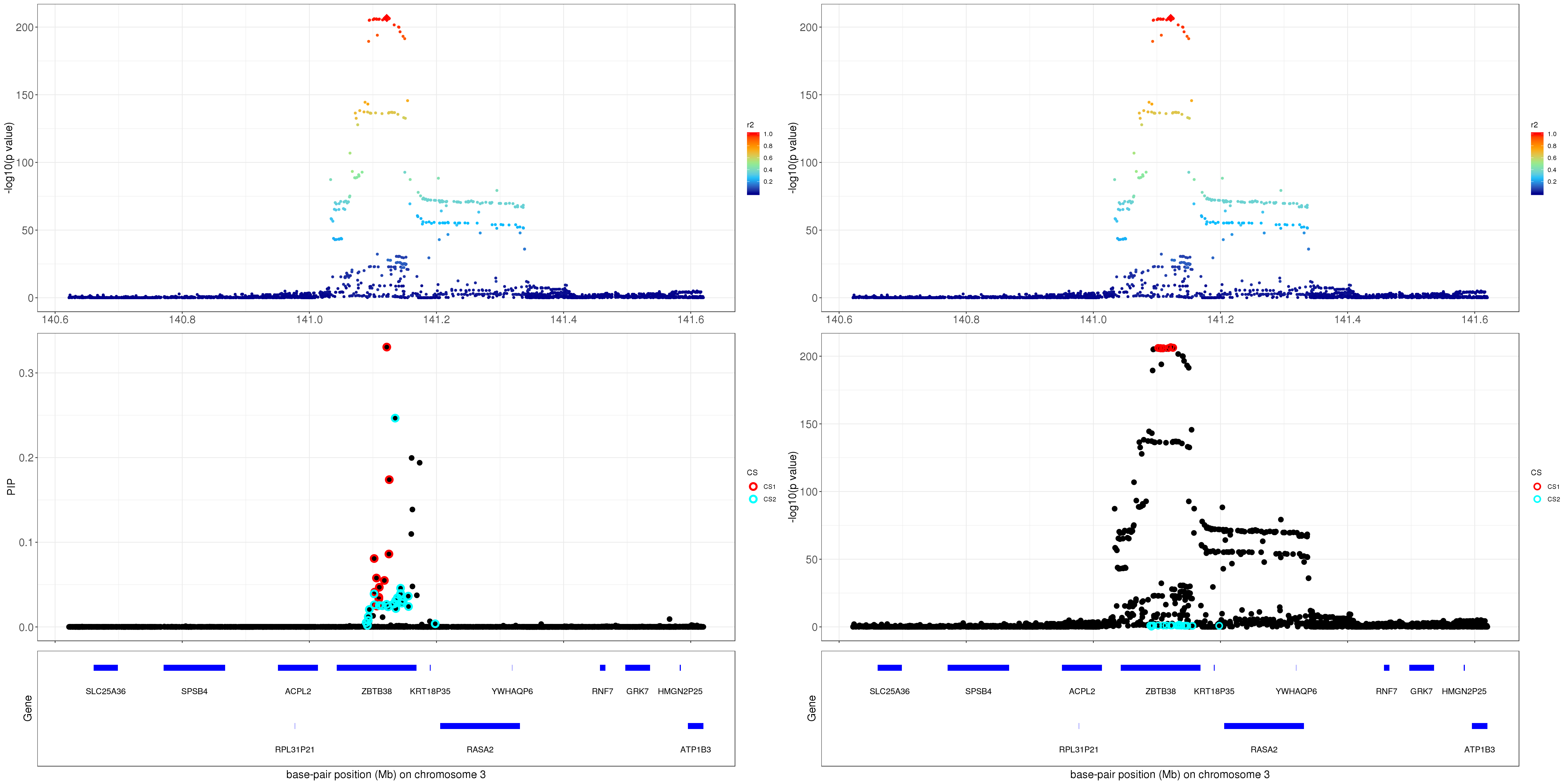
| Version | Author | Date |
|---|---|---|
| 149b7c7 | zouyuxin | 2019-11-19 |
For 1Mb region about ZBTB38, SuSiE found 2 CSs. The SNP with the strongest marginal p value in CS1 is rs2871960 (p = 1.8670e-207). For CS2, the SNP with the strongest marginal p value is rs11919556 (p = 0.0211).
The correlation between rs2871960 and rs11919556 is 0.221051. The average correlation between SNPs in CS1 and CS2 is
round(mean(abs(R[mod_bhat$sets$cs$L1, mod_bhat$sets$cs$L2])), 4)[1] 0.1812Zoom in plot:
p1 = susie_plot_locuszoom(z, mod_bhat, pos = ss.dat$pos$POS/1e6, chr=3, gene.pos.map = gene.pos.map, z.ref.name = names(z), ld = R[z.max,], title='ZBTB38 Credible Sets', plot.locuszoom = FALSE, y.susie = 'p', xrange=c(140.9,141.5), title.size = 20)
p1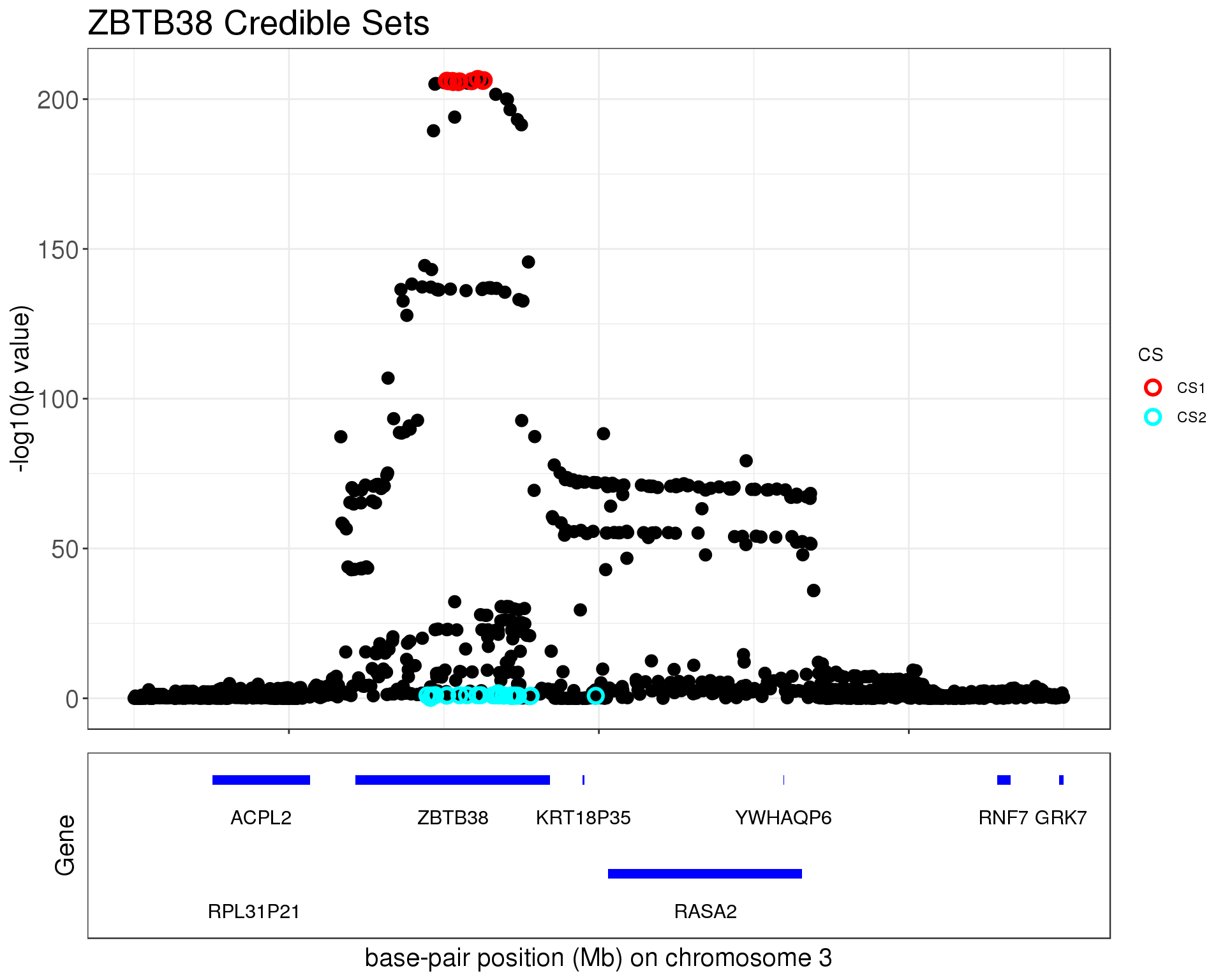
| Version | Author | Date |
|---|---|---|
| 149b7c7 | zouyuxin | 2019-11-19 |
The first credible set contains
cs1 = ss.dat$pos[unlist(mod_bhat$sets$cs$L1),]
cs1$gene = sapply(cs1$POS/1e6, function(i){
  id = intersect(which(gene.pos.map$start <= i), which(gene.pos.map$end >= i))
  gene.pos.map$geneName[id]
})
cs1
#CHROM POS ID REF ALT maf gene
1255 3 141101961 rs9853018 T C 0.446589 ZBTB38
1258 3 141102833 rs6763931 A G 0.446887 ZBTB38
1261 3 141105570 rs724016 G A 0.447055 ZBTB38
1262 3 141106063 rs7632381 C T 0.447588 ZBTB38
1267 3 141109321 rs6808936 G A 0.447482 ZBTB38
1268 3 141109348 rs6785012 T C 0.447476 ZBTB38
1270 3 141110074 rs4683606 G A 0.447216 ZBTB38
1278 3 141118028 rs13068733 G A 0.447268 ZBTB38
1281 3 141121814 rs2871960 C A 0.447921 ZBTB38
1288 3 141125186 rs1344674 G A 0.449007 ZBTB38
1291 3 141125705 rs1344672 G C 0.448705 ZBTB38The second credible set contains
cs2 = ss.dat$pos[unlist(mod_bhat$sets$cs$L2),]
cs2$gene = sapply(cs2$POS/1e6, function(i){
  id = intersect(which(gene.pos.map$start <= i), which(gene.pos.map$end >= i))
  gene.pos.map$geneName[id]
})
cs2
#CHROM POS ID REF ALT maf gene
1225 3 141089418 rs115198977 A C 0.028305 ZBTB38
1226 3 141091356 rs116086535 T G 0.039387 ZBTB38
1230 3 141092497 rs55675250 C T 0.028124 ZBTB38
1231 3 141092645 rs56259972 T A 0.028307 ZBTB38
1234 3 141094334 rs77022697 T C 0.027163 ZBTB38
1253 3 141101781 rs80060248 C G 0.027312 ZBTB38
1256 3 141102130 rs118108151 A G 0.027106 ZBTB38
1269 3 141110025 rs79361824 G A 0.027174 ZBTB38
1275 3 141114894 rs75828411 A G 0.027178 ZBTB38
1280 3 141121557 rs117589471 C G 0.027313 ZBTB38
1284 3 141123883 rs117323650 T C 0.027176 ZBTB38
1301 3 141131707 rs75092195 A G 0.027288 ZBTB38
1303 3 141133260 rs74441190 A G 0.027288 ZBTB38
1312 3 141135004 rs11919556 C T 0.041658 ZBTB38
1315 3 141135690 rs114626934 G A 0.027292 ZBTB38
1317 3 141136022 rs6440005 C T 0.027713 ZBTB38
1324 3 141138545 rs115126368 C T 0.027296 ZBTB38
1325 3 141138692 rs144648746 A G 0.027296 ZBTB38
1344 3 141143205 rs79057647 C T 0.027288 ZBTB38
1347 3 141143489 rs77828701 C T 0.025980 ZBTB38
1348 3 141143491 rs76300426 T C 0.026070 ZBTB38
1350 3 141143620 rs79197573 G A 0.027285 ZBTB38
1360 3 141145479 rs79311431 G A 0.027700 ZBTB38
1361 3 141145601 rs79153193 A C 0.027680 ZBTB38
1366 3 141147784 rs115605995 A C 0.027669 ZBTB38
1390 3 141155631 rs140143440 T C 0.027114 ZBTB38
1391 3 141156007 rs114802788 T C 0.027317 ZBTB38
1474 3 141197995 rs116215663 C A 0.025722 CS 1
- Option 1. We remove effect of top SNP in CS 2.
library(data.table)
library(readr)
library(Matrix)
geno.file = 'height.ZBTB38.raw.gz'
cat("Reading genotype data.\n")
geno <- fread(geno.file,sep = "\t",header = TRUE,stringsAsFactors = FALSE)
class(geno) <- "data.frame"

# Extract the genotypes.
X <- as(as.matrix(geno[-(1:6)]),'dgCMatrix')

pheno.file <- "/gpfs/data/stephens-lab/finemap-uk-biobank/data/raw/height.csv.gz"
out.pheno.file <- "pheno.height.txt"
out.covar.file <- "covar.removeCS2.height.txt"

# LOAD PHENOTYPE and COVARIATES DATA
# -------------------
# Read the phenotype data from the CSV file.
cat("Reading phenotype data.\n")
pheno        <- suppressMessages(read_csv(pheno.file))
class(pheno) <- "data.frame"
pheno$sex = factor(pheno$sex)
pheno$assessment_centre = factor(pheno$assessment_centre)
pheno$genotype_measurement_batch = factor(pheno$genotype_measurement_batch)
pheno$age2 = pheno$age^2
# match individual order with genotype file
ind = fread('height.ZBTB38.psam')
match.idx = match(ind$IID, pheno$id)
pheno = pheno[match.idx,]

Z = model.matrix(~ sex + age + age2 + assessment_centre + genotype_measurement_batch +
                   pc_genetic1 + pc_genetic2 + pc_genetic3 + pc_genetic4 + pc_genetic5 +
                   pc_genetic6 + pc_genetic7 + pc_genetic8 + pc_genetic9 + pc_genetic10 +
                   pc_genetic11 + pc_genetic12 + pc_genetic13 + pc_genetic14 + pc_genetic15 +
                   pc_genetic16 + pc_genetic17 + pc_genetic18 + pc_genetic19 + pc_genetic20 + X[,1312], data = pheno)

# Remove intercept
Z = Z[,-1]
colnames(Z)[150] = 'X'
Z = scale(Z, center=T, scale=F)
# standardize quantitative columns
cols = which(colnames(Z) %in% c("age","pc_genetic1","pc_genetic2","pc_genetic3","pc_genetic4",
                                "pc_genetic5","pc_genetic6","pc_genetic7","pc_genetic8","pc_genetic9",
                                "pc_genetic10","pc_genetic11","pc_genetic12","pc_genetic13","pc_genetic14",
                                "pc_genetic15","pc_genetic16","pc_genetic17","pc_genetic18","pc_genetic19","pc_genetic20"))
Z[,cols] = scale(Z[,cols])
Z[,'age2'] = Z[,'age']^2

# Compute XtX and Xty
y = pheno$height
names(y) = pheno$id

# Center y
y = y - mean(y)
# Center X
X = scale(X, center=T, scale=FALSE)
xtxdiag = colSums(X^2)

A   <- crossprod(Z) # Z'Z
# chol decomposition for (Z'Z)^(-1)
R = chol(solve(A)) # R'R = (Z'Z)^(-1)
W = R %*% crossprod(Z, X) # RZ'X
S = R %*% crossprod(Z, y) # RZ'y

# Load LD matrix from raw genotype
ld.matrix = as.matrix(fread(paste0('height.ZBTB38.matrix')))
# X'X
XtX = sqrt(xtxdiag) * t(ld.matrix*sqrt(xtxdiag)) - crossprod(W) # W'W = X'ZR'RZ'X = X'Z(Z'Z)^{-1}Z'X
rownames(XtX) = colnames(XtX) = colnames(X)
# X'y
Xty = as.vector(y %*% X)
Xty = Xty - crossprod(W, S) # W'S = X'ZR'RZ'y = X'Z(Z'Z)^{-1}Z'y

## SNP info
maf <- read.delim('height.ZBTB38.afreq')
pos <- fread('height.ZBTB38.pvar')
pos$maf = pmin(maf$ALT_FREQS, 1-maf$ALT_FREQS)

saveRDS(list(XtX = XtX, Xty = Xty, yty = sum(y^2) - crossprod(S), n = length(y), pos=pos),
        paste0('height.ZBTB38.removeCS2.XtX.Xty.rds'))
After removing the effect of rs11919556 (p = 0.0211), the p values and z scores are plotted below. The color is correspongding to LD, the shape is corresponding to CS. The SNP in CS is labeled with filled circle.
ss.dat = readRDS('output/height.ZBTB38.removeCS2.XtX.Xty.rds')
betas = as.vector(ss.dat$Xty/diag(ss.dat$XtX))
rss = c(ss.dat$yty) - betas * ss.dat$Xty
se = as.vector(sqrt(rss/((ss.dat$n-1)*diag(ss.dat$XtX))))
z = betas/se
pval = 2*pnorm(-abs(z))
R = as.matrix(t(ss.dat$XtX * (1/sqrt(diag(ss.dat$XtX)))) * (1/ sqrt(diag(ss.dat$XtX))))
names(z) = rownames(R)
z.max = which.max(abs(z))
p1 = locus.zoom.cs(z, cs = mod_bhat$sets$cs$L1, pos=ss.dat$pos$POS/1e6, chr=3, gene.pos.map = gene.pos.map, z.ref.name = names(z)[z.max], ld = R[z.max,], xrange=c(140.9,141.5), title='ZBTB38 CS1', y.lab = '-log10(p value condition on CS2)')
p2 = locus.zoom.cs(z, cs = mod_bhat$sets$cs$L1, pos=ss.dat$pos$POS/1e6, chr=3, gene.pos.map = gene.pos.map, z.ref.name = names(z)[z.max], ld = R[z.max,], xrange=c(140.9,141.5), title='ZBTB38 CS1', y.lab = 'z scores condition on CS2', y.type = 'z')
grid.arrange(p1, p2, ncol=2)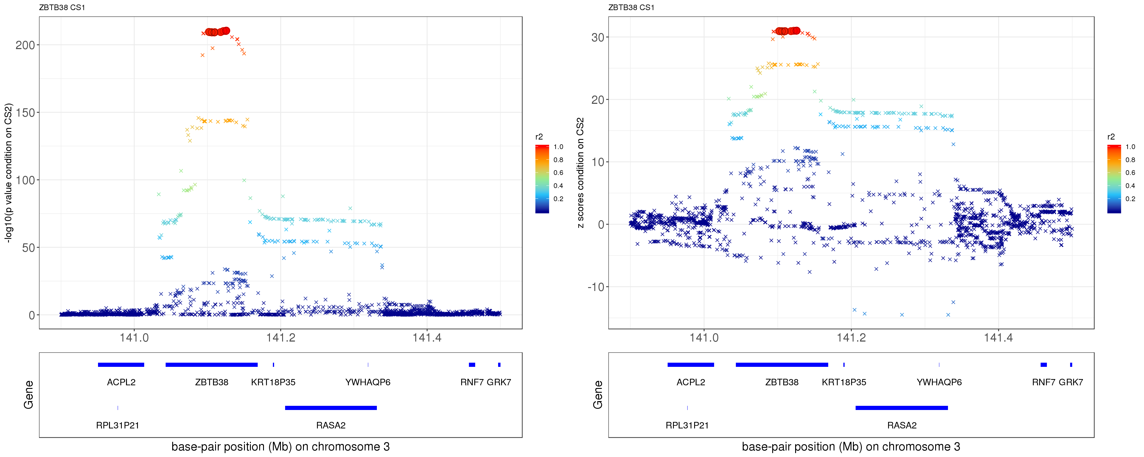
| Version | Author | Date |
|---|---|---|
| 149b7c7 | zouyuxin | 2019-11-19 |
- Option 2. We remove effect of all other CSs.
Instead of removing the effect of top SNP from other CSs, we do exactly what SuSiE does here. In SuSiE, we estimate effects using residuals that are obtained by removing the effects of all other CSs.
The residuals after removing the effects from CSs other than CS1 is \[ r = y - \mathbf{X} \sum_{l=2}^{L}\hat{\mathbf{b}}_{l}. \]
ss.dat = readRDS('data/height.ZBTB38.XtX.Xty.rds')
XtX.scale = t(ss.dat$XtX / mod_bhat$X_column_scale_factors) / mod_bhat$X_column_scale_factors
XtXr = mod_bhat$XtXr - XtX.scale %*% (mod_bhat$alpha[1,] * mod_bhat$mu[1,])
Xtr = ss.dat$Xty/mod_bhat$X_column_scale_factors - XtXr
betas = Xtr/diag(XtX.scale)
b_2 = colSums(mod_bhat$alpha[-1,]*mod_bhat$mu[-1,])
rss = c(ss.dat$yty - 2*sum(ss.dat$Xty * b_2) + sum(XtXr * b_2)) - betas * Xtr
se = as.vector(sqrt(rss/((ss.dat$n-1)*diag(XtX.scale))))
z.CS1 = betas/se
R = as.matrix(t(ss.dat$XtX * (1/sqrt(diag(ss.dat$XtX)))) * (1/ sqrt(diag(ss.dat$XtX))))
names(z.CS1) = colnames(R)
z.cs1.max = which.max(abs(z.CS1))
p1 = locus.zoom.cs(z.CS1, mod_bhat$sets$cs$L1, pos=ss.dat$pos$POS/1e6, chr = 3, gene.pos.map = gene.pos.map, z.ref.name = names(z.cs1.max), ld = R[z.cs1.max,], xrange=c(140.9,141.5), title='ZBTB38 Credible Set 1', y.lab = '-log10(p value condition on other CSs)', title.size = 20)
p2 = locus.zoom.cs(z.CS1, mod_bhat$sets$cs$L1, pos=ss.dat$pos$POS/1e6, chr = 3, gene.pos.map = gene.pos.map, z.ref.name = names(z.cs1.max), ld = R[z.cs1.max,], xrange=c(140.9,141.5), title='ZBTB38 Credible Set 1', y.lab = 'z scores condition on other CSs', title.size = 20, y.type='z')
grid.arrange(p1, p2, ncol=2)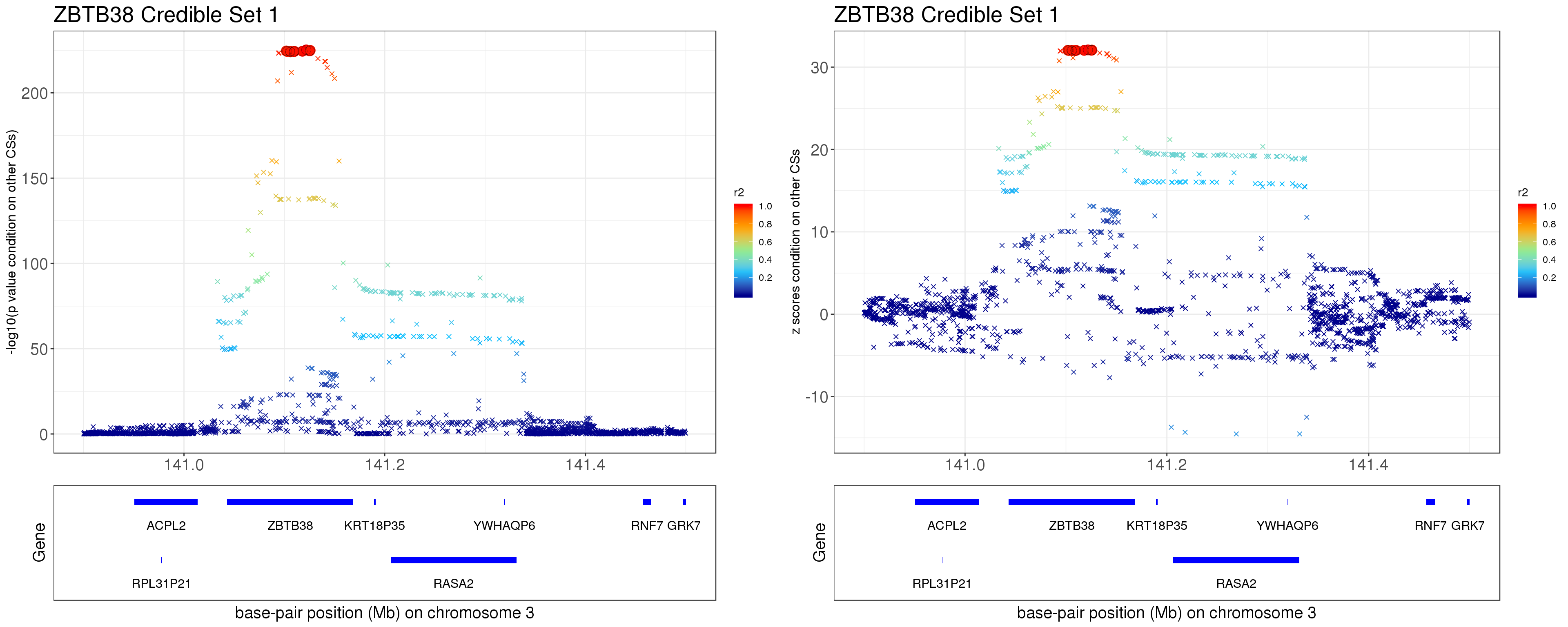
| Version | Author | Date |
|---|---|---|
| 149b7c7 | zouyuxin | 2019-11-19 |
CS 2
- Option 1. We remove effect of top SNP in CS 1.
library(data.table)
library(readr)
library(Matrix)
geno.file = 'height.ZBTB38.raw.gz'
cat("Reading genotype data.\n")
geno <- fread(geno.file,sep = "\t",header = TRUE,stringsAsFactors = FALSE)
class(geno) <- "data.frame"

# Extract the genotypes.
X <- as(as.matrix(geno[-(1:6)]),'dgCMatrix')

pheno.file <- "/gpfs/data/stephens-lab/finemap-uk-biobank/data/raw/height.csv.gz"
out.pheno.file <- "pheno.height.txt"
out.covar.file <- "covar.removeCS1.height.txt"

# LOAD PHENOTYPE and COVARIATES DATA
# -------------------
# Read the phenotype data from the CSV file.
cat("Reading phenotype data.\n")
pheno        <- suppressMessages(read_csv(pheno.file))
class(pheno) <- "data.frame"
pheno$sex = factor(pheno$sex)
pheno$assessment_centre = factor(pheno$assessment_centre)
pheno$genotype_measurement_batch = factor(pheno$genotype_measurement_batch)
pheno$age2 = pheno$age^2
# match individual order with genotype file
ind = fread('height.ZBTB38.psam')
match.idx = match(ind$IID, pheno$id)
pheno = pheno[match.idx,]

Z = model.matrix(~ sex + age + age2 + assessment_centre + genotype_measurement_batch +
                   pc_genetic1 + pc_genetic2 + pc_genetic3 + pc_genetic4 + pc_genetic5 +
                   pc_genetic6 + pc_genetic7 + pc_genetic8 + pc_genetic9 + pc_genetic10 +
                   pc_genetic11 + pc_genetic12 + pc_genetic13 + pc_genetic14 + pc_genetic15 +
                   pc_genetic16 + pc_genetic17 + pc_genetic18 + pc_genetic19 + pc_genetic20 + X[,1281], data = pheno)

# Remove intercept
Z = Z[,-1]
colnames(Z)[150] = 'X'
Z = scale(Z, center=T, scale = F)
# standardize quantitative columns
cols = which(colnames(Z) %in% c("age","pc_genetic1","pc_genetic2","pc_genetic3","pc_genetic4",
                                "pc_genetic5","pc_genetic6","pc_genetic7","pc_genetic8","pc_genetic9",
                                "pc_genetic10","pc_genetic11","pc_genetic12","pc_genetic13","pc_genetic14",
                                "pc_genetic15","pc_genetic16","pc_genetic17","pc_genetic18","pc_genetic19","pc_genetic20"))
Z[,cols] = scale(Z[,cols])
Z[,'age2'] = Z[,'age']^2

# Compute XtX and Xty
y = pheno$height
names(y) = pheno$id

# Center y
y = y - mean(y)
# Center X
X = scale(X, center=TRUE, scale = FALSE)
xtxdiag = colSums(X^2)

A   <- crossprod(Z) # Z'Z
# chol decomposition for (Z'Z)^(-1)
R = chol(solve(A)) # R'R = (Z'Z)^(-1)
W = R %*% crossprod(Z, X) # RZ'X
S = R %*% crossprod(Z, y) # RZ'y

# Load LD matrix from raw genotype
ld.matrix = as.matrix(fread(paste0('height.ZBTB38.matrix')))
# X'X
XtX = sqrt(xtxdiag) * t(ld.matrix*sqrt(xtxdiag)) - crossprod(W) # W'W = X'ZR'RZ'X = X'Z(Z'Z)^{-1}Z'X
rownames(XtX) = colnames(XtX) = colnames(X)
# X'y
Xty = as.vector(y %*% X)
Xty = Xty - crossprod(W, S) # W'S = X'ZR'RZ'y = X'Z(Z'Z)^{-1}Z'y

## SNP info
maf <- read.delim('height.ZBTB38.afreq')
pos <- fread('height.ZBTB38.pvar')
pos$maf = pmin(maf$ALT_FREQS, 1-maf$ALT_FREQS)

saveRDS(list(XtX = XtX, Xty = Xty, yty = sum(y^2) - crossprod(S), n = length(y), pos=pos),
        paste0('height.ZBTB38.removeCS1.XtX.Xty.rds'))
After removing the effect of rs2871960 (p = 1.8674e-207), the conditional p value for rs11919556 becomes 4.279e-06, and it becomes the strongest one among all SNPs!
ss.dat = readRDS('output/height.ZBTB38.removeCS1.XtX.Xty.rds')
betas = as.vector(ss.dat$Xty/diag(ss.dat$XtX))
rss = c(ss.dat$yty) - betas * ss.dat$Xty
se = as.vector(sqrt(rss/((ss.dat$n-1)*diag(ss.dat$XtX))))
z = betas/se
pval = 2*pnorm(-abs(z))
R = as.matrix(t(ss.dat$XtX * (1/sqrt(diag(ss.dat$XtX)))) * (1/ sqrt(diag(ss.dat$XtX))))
names(z) = rownames(R)
z.max = which.max(abs(z))
p1 = locus.zoom.cs(z, cs = mod_bhat$sets$cs$L2, pos=ss.dat$pos$POS/1e6, chr=3, gene.pos.map = gene.pos.map, z.ref.name = names(z)[z.max], ld = R[z.max,], xrange=c(140.9,141.5), title='ZBTB38 CS2', y.lab = '-log10(p value condition on CS1)')
p2 = locus.zoom.cs(z, cs = mod_bhat$sets$cs$L2, pos=ss.dat$pos$POS/1e6, chr=3, gene.pos.map = gene.pos.map, z.ref.name = names(z)[z.max], ld = R[z.max,], xrange=c(140.9,141.5), title='ZBTB38 CS2', y.lab = 'z scores condition on CS1', y.type = 'z')
grid.arrange(p1, p2, ncol=2)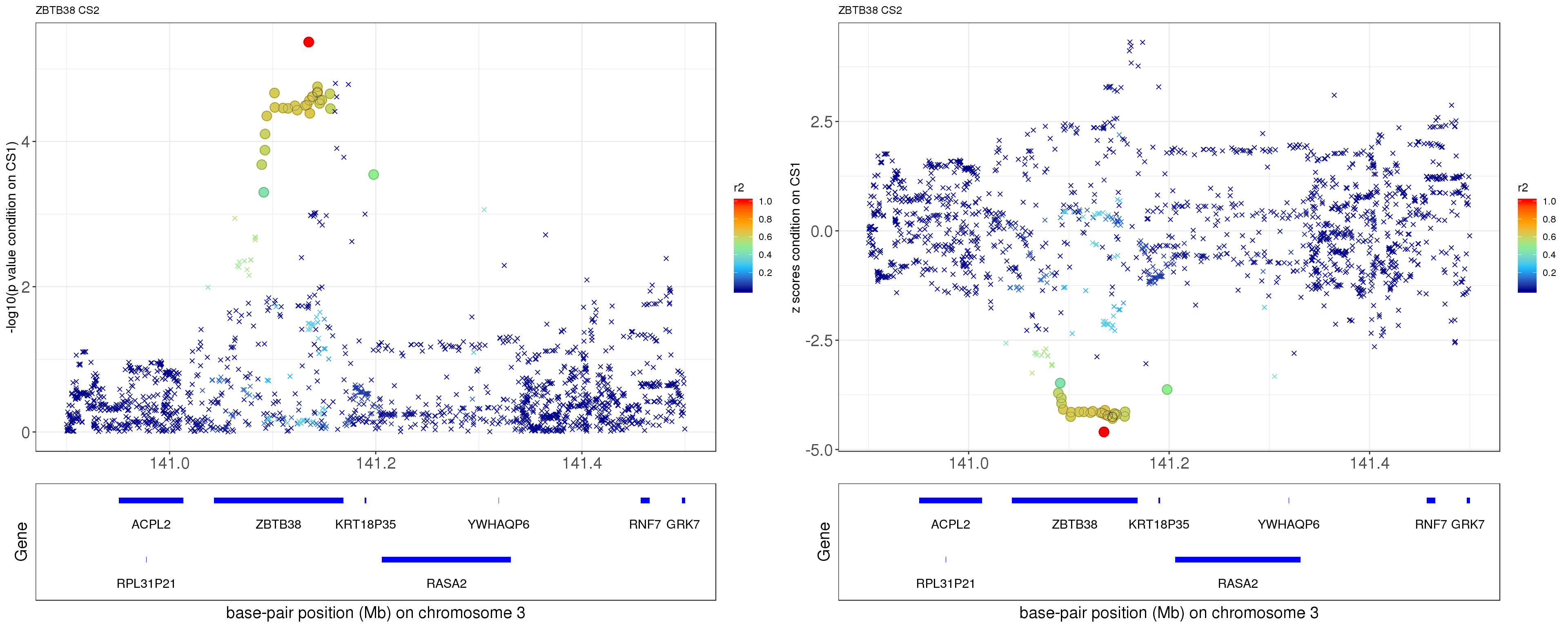
| Version | Author | Date |
|---|---|---|
| 149b7c7 | zouyuxin | 2019-11-19 |
- Option 2. We remove effect of all other CSs.
Instead of removing the effect of top SNP from other CSs, we do exactly what SuSiE does here. In SuSiE, we estimate effects using residuals that are obtained by removing the effects of all other CSs.
The residuals after removing the effects from CSs other than CS2 is \[ r = y - \mathbf{X} \sum_{l\neq 2}^{L}\hat{\mathbf{b}}_{l}. \]
ss.dat = readRDS('data/height.ZBTB38.XtX.Xty.rds')
XtX.scale = t(ss.dat$XtX / mod_bhat$X_column_scale_factors) / mod_bhat$X_column_scale_factors
XtXr = mod_bhat$XtXr - XtX.scale %*% (mod_bhat$alpha[2,] * mod_bhat$mu[2,])
Xtr = ss.dat$Xty/mod_bhat$X_column_scale_factors - XtXr
betas = Xtr/diag(XtX.scale)
b_2 = colSums(mod_bhat$alpha[-2,]*mod_bhat$mu[-2,])
rss = c(ss.dat$yty - 2*sum(ss.dat$Xty * b_2) + sum(XtXr * b_2)) - betas * Xtr
se = as.vector(sqrt(rss/((ss.dat$n-1)*diag(XtX.scale))))
z.CS2 = betas/se
R = as.matrix(t(ss.dat$XtX * (1/sqrt(diag(ss.dat$XtX)))) * (1/ sqrt(diag(ss.dat$XtX))))
names(z.CS2) = colnames(R)
z.cs2.max = which.max(abs(z.CS2))
p1 = locus.zoom.cs(z.CS2, mod_bhat$sets$cs$L2, pos=ss.dat$pos$POS/1e6, chr = 3, gene.pos.map = gene.pos.map, z.ref.name = names(z.cs2.max), ld = R[z.cs2.max,], xrange=c(140.9,141.5), title='ZBTB38 Credible Set 2', y.lab = '-log10(p value condition on other CSs)', title.size = 20)
p2 = locus.zoom.cs(z.CS2, mod_bhat$sets$cs$L2, pos=ss.dat$pos$POS/1e6, chr = 3, gene.pos.map = gene.pos.map, z.ref.name = names(z.cs2.max), ld = R[z.cs2.max,], xrange=c(140.9,141.5), title='ZBTB38 Credible Set 2', y.lab = 'z scores condition on other CSs', title.size = 20, y.type='z')
grid.arrange(p1, p2, ncol=2)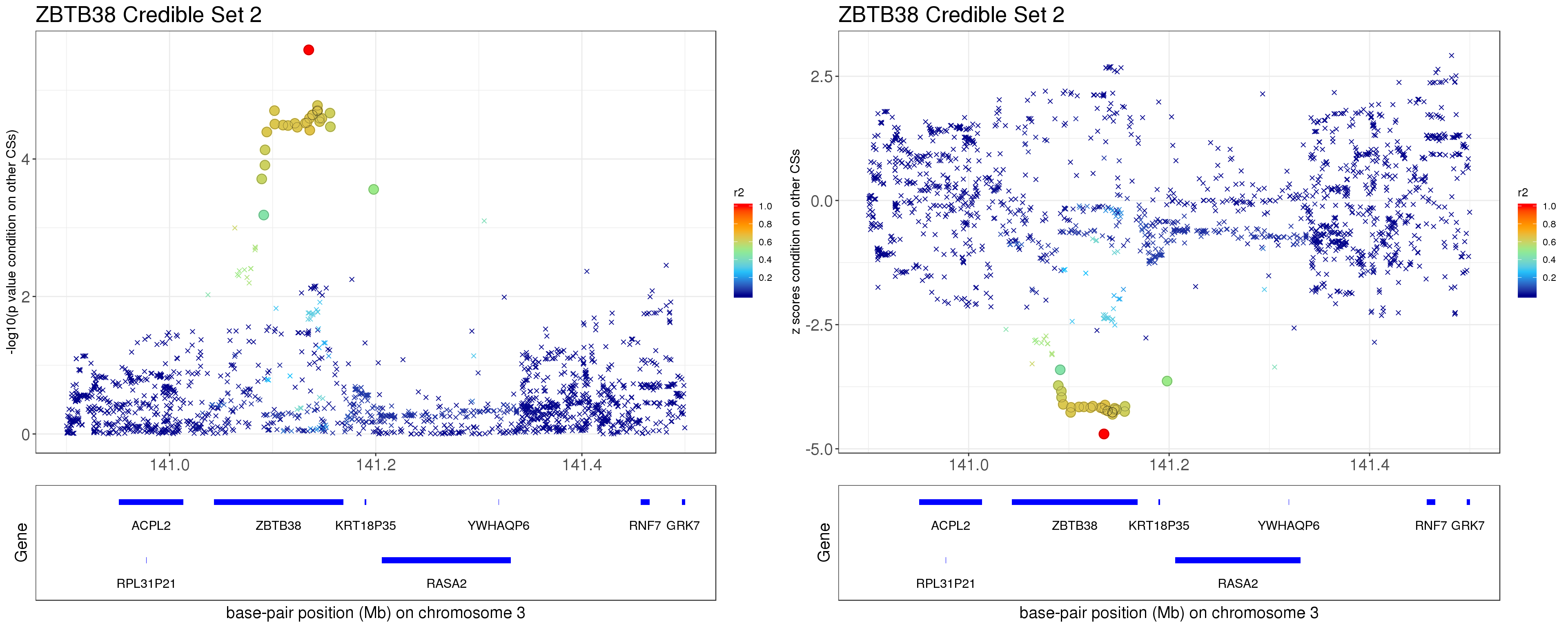
Simulation under the estimated model
In the following simulation, we treat rs2871960 and rs11919556 as true signals. The effect sizes are from estimated model. We use the fitted residual variance in the simulation. The response y is simulated from \[ y \sim N_n(Xb, \sigma^2 I) \] , where X the genotype matrix that column centered, scaled, and removed the effect of covariates.
# ON CRI
library(data.table)
library(readr)
library(Matrix)
library(susieR)
geno.file = 'height.ZBTB38.raw.gz'
cat("Reading genotype data.\n")
geno <- fread(geno.file,sep = "\t",header = TRUE,stringsAsFactors = FALSE)
class(geno) <- "data.frame"

# Extract the genotypes.
X <- as(as.matrix(geno[-(1:6)]),'dgCMatrix')

pheno.file <- "/gpfs/data/stephens-lab/finemap-uk-biobank/data/raw/height.csv.gz"

# LOAD PHENOTYPE and COVARIATES DATA
# -------------------
# Read the phenotype data from the CSV file.
cat("Reading phenotype data.\n")
pheno        <- suppressMessages(read_csv(pheno.file))
class(pheno) <- "data.frame"
pheno$sex = factor(pheno$sex)
pheno$assessment_centre = factor(pheno$assessment_centre)
pheno$genotype_measurement_batch = factor(pheno$genotype_measurement_batch)
pheno$age2 = pheno$age^2
# match individual order with genotype file
ind = fread('height.ZBTB38.psam')
match.idx = match(ind$IID, pheno$id)
pheno = pheno[match.idx,]

Z = model.matrix(~ sex + age + age2 + assessment_centre + genotype_measurement_batch +
                   pc_genetic1 + pc_genetic2 + pc_genetic3 + pc_genetic4 + pc_genetic5 +
                   pc_genetic6 + pc_genetic7 + pc_genetic8 + pc_genetic9 + pc_genetic10 +
                   pc_genetic11 + pc_genetic12 + pc_genetic13 + pc_genetic14 + pc_genetic15 +
                   pc_genetic16 + pc_genetic17 + pc_genetic18 + pc_genetic19 + pc_genetic20, data = pheno)

# Remove intercept
Z = Z[,-1]
Z = scale(Z, center=TRUE, scale=FALSE)
# standardize quantitative columns
cols = which(colnames(Z) %in% c("age","pc_genetic1","pc_genetic2","pc_genetic3","pc_genetic4",
                                "pc_genetic5","pc_genetic6","pc_genetic7","pc_genetic8","pc_genetic9",
                                "pc_genetic10","pc_genetic11","pc_genetic12","pc_genetic13","pc_genetic14",
                                "pc_genetic15","pc_genetic16","pc_genetic17","pc_genetic18","pc_genetic19","pc_genetic20"))
Z[,cols] = scale(Z[,cols])
Z[,'age2'] = Z[,'age']^2

# Center X
X = scale(X, center=TRUE, scale = FALSE)
xtxdiag = colSums(X^2)

A   <- crossprod(Z)
# chol decomposition for (Z'Z)^(-1)
R = chol(solve(A))
W = R %*% t(Z) %*% X

# Remove Covariates from X
X   <- as.matrix(X - Z %*% crossprod(R,W))

# Get estimated parameters
ss.dat = readRDS('height.ZBTB38.XtX.Xty.rds')
betas = as.vector(ss.dat$Xty)/diag(ss.dat$XtX)
rss = c(ss.dat$yty) - betas * ss.dat$Xty
se = as.vector(sqrt(rss/((ss.dat$n-1)*diag(ss.dat$XtX))))
R = as.matrix(t(ss.dat$XtX * (1/sqrt(diag(ss.dat$XtX)))) * (1/ sqrt(diag(ss.dat$XtX))))
mod_bhat.ld = susie_bhat(bhat = betas, shat = se, R = R, n = ss.dat$n, var_y = as.numeric(ss.dat$yty/(ss.dat$n-1)), standardize = T)
sigma2 = mod_bhat.ld$sigma2
b2 = c(mod_bhat.ld$mu[1, 1281], mod_bhat.ld$mu[2, 1312])/mod_bhat.ld$X_column_scale_factors[1281, 1312]
Xb = as.vector(X[, c(1281, 1312)] %*% b2)

n = nrow(X)
result = vector("list", 1000)
set.seed(201910)
for(i in 1:1000){
  ## generate y
  y = Xb + rnorm(n, 0, sqrt(sigma2))

  ## compute Xty, yty
  Xty = as.vector(y %*% X)
  yty = sum(y^2)

  ## compute summary stats
  betas = as.vector(Xty/diag(ss.dat$XtX))
  rss = yty - betas * Xty
  se = as.vector(sqrt(rss/((n-1)*diag(ss.dat$XtX))))
  z = betas/se

  result[[i]] = susie_bhat(betas, se, R=R, n=n, var_y = as.numeric(yty/(n-1)), standardize = T)
}
saveRDS(result, 'height.ZBTB38.simulation1000.rds')
Load simulation results:
result = readRDS('output/height.ZBTB38.simulation1000.rds')In 1000 simulations, 320 runs have 2 CSs. The rests have 1 CS.
table(sapply(result, function(mod) length(mod$sets$cs)))
  1   2
680 320
291 runs contain both true signals.
contain.true = sapply(result, function(mod) all(c(1281, 1312) %in% unlist(mod$sets$cs)))
sum(contain.true)
[1] 291963 runs contain rs2871960.
contain.true.1 = sapply(result, function(mod) all( 1281 %in% unlist(mod$sets$cs)))
sum(contain.true.1)
[1] 963302 runs contain rs11919556.
contain.true.2 = sapply(result, function(mod) all( 1312 %in% unlist(mod$sets$cs)))
sum(contain.true.2)
[1] 302
sessionInfo()R version 3.5.1 (2018-07-02)
Platform: x86_64-pc-linux-gnu (64-bit)
Running under: Scientific Linux 7.4 (Nitrogen)
Matrix products: default
BLAS/LAPACK: /software/openblas-0.2.19-el7-x86_64/lib/libopenblas_haswellp-r0.2.19.so
locale:
[1] LC_CTYPE=en_US.UTF-8 LC_NUMERIC=C
[3] LC_TIME=en_US.UTF-8 LC_COLLATE=en_US.UTF-8
[5] LC_MONETARY=en_US.UTF-8 LC_MESSAGES=en_US.UTF-8
[7] LC_PAPER=en_US.UTF-8 LC_NAME=C
[9] LC_ADDRESS=C LC_TELEPHONE=C
[11] LC_MEASUREMENT=en_US.UTF-8 LC_IDENTIFICATION=C
attached base packages:
[1] stats graphics grDevices utils datasets methods base
other attached packages:
[1] ggplot2_3.1.1 susieR_0.8.1.0545 gridExtra_2.3 dplyr_0.8.0.1
[5] readr_1.3.1
loaded via a namespace (and not attached):
[1] Rcpp_1.0.1 plyr_1.8.4 pillar_1.3.1 compiler_3.5.1
[5] later_0.7.5 git2r_0.26.1 workflowr_1.5.0 tools_3.5.1
[9] digest_0.6.18 evaluate_0.12 tibble_2.0.1 gtable_0.2.0
[13] lattice_0.20-38 egg_0.4.5 pkgconfig_2.0.2 rlang_0.3.1
[17] Matrix_1.2-15 yaml_2.2.0 withr_2.1.2 stringr_1.3.1
[21] knitr_1.20 fs_1.3.1 hms_0.4.2 rprojroot_1.3-2
[25] grid_3.5.1 tidyselect_0.2.5 glue_1.3.0 R6_2.3.0
[29] rmarkdown_1.10 purrr_0.3.2 magrittr_1.5 whisker_0.3-2
[33] backports_1.1.2 scales_1.0.0 promises_1.0.1 htmltools_0.3.6
[37] assertthat_0.2.1 colorspace_1.4-0 httpuv_1.4.5 labeling_0.3
[41] stringi_1.2.4 lazyeval_0.2.1 munsell_0.5.0 crayon_1.3.4