Examine methylation and H3K27ac fine-mapping results from the ROSMAP data
William Denault, Hao Sun, Angjing Liu, Peter Carbonetto, Gao Wang
Last updated: 2025-03-20
Checks: 7 0
Knit directory:
fsusie-experiments/analysis/
This reproducible R Markdown analysis was created with workflowr (version 1.7.1). The Checks tab describes the reproducibility checks that were applied when the results were created. The Past versions tab lists the development history.
Great! Since the R Markdown file has been committed to the Git repository, you know the exact version of the code that produced these results.
Great job! The global environment was empty. Objects defined in the global environment can affect the analysis in your R Markdown file in unknown ways. For reproduciblity it’s best to always run the code in an empty environment.
The command set.seed(1) was run prior to running the
code in the R Markdown file. Setting a seed ensures that any results
that rely on randomness, e.g. subsampling or permutations, are
reproducible.
Great job! Recording the operating system, R version, and package versions is critical for reproducibility.
Nice! There were no cached chunks for this analysis, so you can be confident that you successfully produced the results during this run.
Great job! Using relative paths to the files within your workflowr project makes it easier to run your code on other machines.
Great! You are using Git for version control. Tracking code development and connecting the code version to the results is critical for reproducibility.
The results in this page were generated with repository version 1ad355a. See the Past versions tab to see a history of the changes made to the R Markdown and HTML files.
Note that you need to be careful to ensure that all relevant files for
the analysis have been committed to Git prior to generating the results
(you can use wflow_publish or
wflow_git_commit). workflowr only checks the R Markdown
file, but you know if there are other scripts or data files that it
depends on. Below is the status of the Git repository when the results
were generated:
Untracked files:
    Untracked:  data/analysis_result/Fungen_xQTL.ENSG00000163808.cis_results_db.export.rds
    Untracked:  data/analysis_result/ROSMAP_haQTL.chr3_43915257_48413435.fsusie_mixture_normal_top_pc_weights.rds
    Untracked:  data/analysis_result/ROSMAP_mQTL.chr3_43915257_48413435.fsusie_mixture_normal_top_pc_weights.rds
    Untracked:  outputs/ROSMAP_haQTL_cs_snp_annotation.tsv.gz
    Untracked:  outputs/ROSMAP_haQTL_cs_snp_toppc1_annotation.tsv.gz
    Untracked:  outputs/ROSMAP_mQTL_cs_snp_annotation.tsv.gz
    Untracked:  outputs/ROSMAP_mQTL_cs_snp_toppc1_annotation.tsv.gz
Note that any generated files, e.g. HTML, png, CSS, etc., are not included in this status report because it is ok for generated content to have uncommitted changes.
These are the previous versions of the repository in which changes were
made to the R Markdown (analysis/rosmap_overview.Rmd) and
HTML (docs/rosmap_overview.html) files. If you’ve
configured a remote Git repository (see ?wflow_git_remote),
click on the hyperlinks in the table below to view the files as they
were in that past version.
| File | Version | Author | Date | Message |
|---|---|---|---|---|
| Rmd | 1ad355a | Peter Carbonetto | 2025-03-20 | wflow_publish("rosmap_overview.Rmd", view = FALSE, verbose = TRUE) |
| html | c84e5c0 | Peter Carbonetto | 2025-03-20 | Rebuilt the rosmap_overview analysis with the new results. |
| Rmd | 1c8eeb7 | Peter Carbonetto | 2025-03-20 | wflow_publish("rosmap_overview.Rmd", view = FALSE) |
| Rmd | acfadd1 | Peter Carbonetto | 2025-03-20 | Made a few improvements to the code and text of the rosmap_analysis. |
| Rmd | c102af9 | Peter Carbonetto | 2025-03-20 | Added a scatterplot comparing number of CSs per TAD (susie vs. fsusie). |
| Rmd | 12f2fd3 | Peter Carbonetto | 2025-03-20 | Added some histograms on TAD CS sizes. |
| Rmd | c69e187 | Peter Carbonetto | 2025-03-20 | Created plot showing TAD sizes from the methylation fine-mapping results. |
| Rmd | 2a5c706 | Peter Carbonetto | 2025-03-20 | Added code to the rosmap_overview analysis to load the methylation SNP results. |
| Rmd | c3a01c7 | Peter Carbonetto | 2025-03-20 | Added link for downloading data to rosmap_overview analysis. |
| html | 5c446c0 | Peter Carbonetto | 2025-03-20 | First build of the rosmap_overview analysis. |
| Rmd | 7532908 | Peter Carbonetto | 2025-03-20 | workflowr::wflow_publish("rosmap_overview.Rmd", verbose = TRUE) |
| Rmd | bc6d0a1 | Peter Carbonetto | 2025-03-20 | Started working on rosmap_overview analysis. |
ADD SOME TEXT HERE GIVING AN OVERVIEW OF THIS ANALYSIS.
Note: If you would like to run this analysis on your computer, you will first need to download the fine-mapping outputs. They can be downloaded from here. Once you have downloaded the files, copy them to the “outputs” subdirectory.
Load some packges used in the code below:
library(data.table)
library(ggplot2)
library(cowplot)
Methylation fine-mapping
First I define a helper function for loading the enrichment results:
# The "n" argument specifies the number of "meta data" columns.
# Columns after that are treated as the enrichment results. These
# columns contain only binary data (0 or 1) indicating whether or not
# the genomic feature (genetic variant or molecular trait location)
# is assigned that specific annotation.
read_enrichment_results <- function (filename, n) {
  out <- fread(filename,sep = "\t",stringsAsFactors = FALSE,header = TRUE)
  class(out) <- "data.frame"
  out <- transform(out,chr = factor(chr))
  cols <- seq(n + 1,ncol(out))
  for (i in cols)
    out[[i]] <- factor(out[[i]])
  return(out)
}
Next I load methylation SNP results generated by SuSiE-topPC and fSuSiE:
methyl_snps_susie_file <-
  "../outputs/ROSMAP_mQTL_cs_snp_toppc1_annotation.tsv.gz"
methyl_snps_fsusie_file <- "../outputs/ROSMAP_mQTL_cs_snp_annotation.tsv.gz"
methyl_snps_susie  <- read_enrichment_results(methyl_snps_susie_file,n = 6)
methyl_snps_fsusie <- read_enrichment_results(methyl_snps_fsusie_file,n = 7)
methyl_snps_susie$region <-
  sapply(strsplit(methyl_snps_susie$cs,":",fixed = TRUE),"[[",2)
methyl_snps_susie  <- transform(methyl_snps_susie,
                                region = factor(region),
                                cs     = factor(cs),
                                pc     = factor(pc))
methyl_snps_fsusie <- transform(methyl_snps_fsusie,
                                cs     = factor(cs),
                                region = factor(region),
                                study  = factor(study))
This is the number of fine-mapping regions (TADs) that contained at least one CS in each of the analyses:
nlevels(methyl_snps_susie$region)
nlevels(methyl_snps_fsusie$region)
# [1] 1236
# [1] 1327
This is a function we will use below to get the sizes of the TADs (in Mb):
get_tad_sizes <- function (tads) {
  tads <- strsplit(tads,"_",fixed = TRUE)
  pos0 <- as.numeric(sapply(tads,"[[",2))
  pos1 <- as.numeric(sapply(tads,"[[",3))
  return((pos1 - pos0)/1e6)
}
This plot summarizes the sizes of the TADs that were analyzed by SuSiE-topPC and fSuSiE:
plot_tad_sizes <- function (tads) {
  tad_size <- get_tad_sizes(tads)
  pdat <- data.frame(tad_size = tad_size)
  return(ggplot(pdat,aes(x = tad_size)) +
         geom_histogram(color = "white",fill = "darkblue",bins = 48) +
         labs(x = "size (Mb)",y = "number of TADs") +
         theme_cowplot(font_size = 10))
}
tads <- levels(methyl_snps_fsusie$region)
plot_tad_sizes(tads) +
  scale_x_continuous(limits = c(2,9),breaks = 1:10) +
  scale_y_continuous(breaks = seq(0,100,10))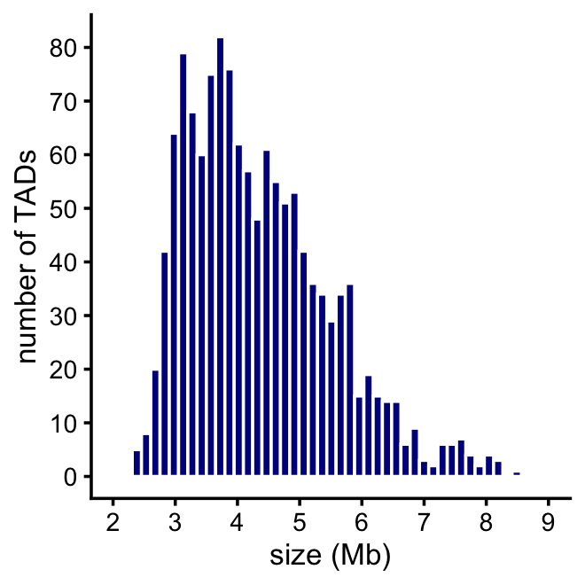
| Version | Author | Date |
|---|---|---|
| c84e5c0 | Peter Carbonetto | 2025-03-20 |
Some more useful statistics on the TAD sizes:
tad_size <- get_tad_sizes(tads)
range(tad_size)
mean(tad_size)
median(tad_size)
sum(tad_size > 9)
# [1]  2.320952 34.727189
# [1] 4.54465
# [1] 4.154266
# [1] 19
These histograms summarize the number of CSs per TAD:
get_cs_vs_tad_size <- function (dat) {
  tads <- levels(dat$region)
  out <- data.frame(tad      = tads,
                    tad_size = get_tad_sizes(tads),
                    num_cs   = tapply(dat$cs,dat$region,
                                      function (x) length(unique(x))))
  rownames(out) <- NULL
  return(out)
}
pdat1 <- get_cs_vs_tad_size(methyl_snps_susie)
pdat2 <- get_cs_vs_tad_size(methyl_snps_fsusie)
pdat1 <- transform(pdat1,num_cs = factor(num_cs,1:20))
pdat2 <- transform(pdat2,num_cs = factor(num_cs,1:20))
p1 <- ggplot(pdat1,aes(x = num_cs)) +
  geom_histogram(stat = "count",color = "white",fill = "darkblue") +
  scale_x_discrete(drop = FALSE) +
  labs(x = "number of CSs",y = "number of TADs",title = "SuSiE-topPC") +
  theme_cowplot(font_size = 10) +
  theme(plot.title = element_text(size = 10,face = "plain"))
p2 <- ggplot(pdat2,aes(x = num_cs)) +
  geom_histogram(stat = "count",color = "white",fill = "darkblue") +
  scale_x_discrete(drop = FALSE) +
  labs(x = "number of CSs",y = "number of TADs",title = "fSuSiE") +
  theme_cowplot(font_size = 10) +
  theme(plot.title = element_text(size = 10,face = "plain"))
plot_grid(p1,p2,nrow = 1,ncol = 2)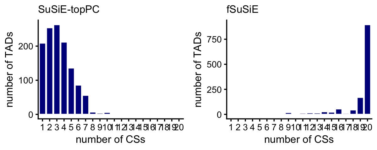
| Version | Author | Date |
|---|---|---|
| c84e5c0 | Peter Carbonetto | 2025-03-20 |
Compare discovery of causal SNPs (number of CSs) in the SuSiE-topPC and fSuSiE analyses:
dat1 <- get_cs_vs_tad_size(methyl_snps_susie)
dat2 <- get_cs_vs_tad_size(methyl_snps_fsusie)
dat1 <- dat1[c(1,3)]
dat2 <- dat2[c(1,3)]
names(dat1) <- c("tad","num_cs_susie")
names(dat2) <- c("tad","num_cs_fsusie")
dat <- merge(dat1,dat2,all = TRUE)
rows <- which(is.na(dat$num_cs_susie))
dat[rows,"num_cs_susie"] <- 0
pdat <- melt(with(dat,table(num_cs_susie,num_cs_fsusie)))
rows <- which(pdat$value == 0)
pdat[rows,"value"] <- NA
ggplot(pdat,aes(x = num_cs_susie,y = num_cs_fsusie,size = value)) +
  geom_point(color = "white",fill = "darkblue",shape = 21) +
  geom_abline(intercept = 0,slope = 1,color = "black",linetype = "dotted") +
  scale_x_continuous(breaks = seq(0,20,2),limits = c(0,20)) +
  scale_y_continuous(breaks = seq(0,20,2),limits = c(0,20)) +
  scale_size(breaks = c(1,10,100)) +
  labs(x = "SuSiE-topPC",y = "fSuSiE",size = "number of TADs") +
  theme_cowplot(font_size = 10)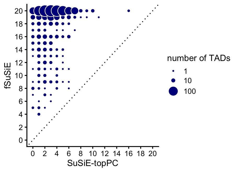
| Version | Author | Date |
|---|---|---|
| c84e5c0 | Peter Carbonetto | 2025-03-20 |
Compare the sizes of the CSs in the SuSiE-topPC and fSuSiE analyses:
bins <- c(0,1,2,5,10,20,Inf)
cs_size_susie  <- as.numeric(table(methyl_snps_susie$cs))
cs_size_fsusie <- as.numeric(table(methyl_snps_fsusie$cs))
cs_size_susie  <- cut(cs_size_susie,bins)
cs_size_fsusie <- cut(cs_size_fsusie,bins)
levels(cs_size_susie) <- bins[-1]
levels(cs_size_fsusie) <- bins[-1]
p1 <- ggplot(data.frame(cs_size = cs_size_susie),aes(x = cs_size)) +
  geom_histogram(stat = "count",color = "white",fill = "darkblue",
                 width = 0.65) +
  labs(x = "CS size",y = "number of CSs",title = "SuSiE-topPC") +
  theme_cowplot(font_size = 10) +
  theme(plot.title = element_text(size = 10,face = "plain"))
p2 <- ggplot(data.frame(cs_size = cs_size_fsusie),aes(x = cs_size)) +
  geom_histogram(stat = "count",color = "white",fill = "darkblue",
                 width = 0.65) +
  labs(x = "CS size",y = "number of CSs",title = "fSuSiE") +
  theme_cowplot(font_size = 10) +
  theme(plot.title = element_text(size = 10,face = "plain"))
plot_grid(p1,p2,nrow = 1,ncol = 2)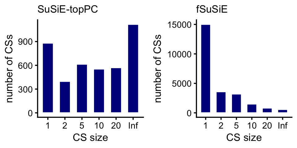
| Version | Author | Date |
|---|---|---|
| c84e5c0 | Peter Carbonetto | 2025-03-20 |
H3K27ac fine-mapping
Load the H3K27ac SNP results generated by SuSiE-topPC and fSuSiE:
ha_snps_susie_file <- "../outputs/ROSMAP_haQTL_cs_snp_toppc1_annotation.tsv.gz"
ha_snps_fsusie_file <- "../outputs/ROSMAP_haQTL_cs_snp_annotation.tsv.gz"
ha_snps_susie  <- read_enrichment_results(ha_snps_susie_file,n = 6)
ha_snps_fsusie <- read_enrichment_results(ha_snps_fsusie_file,n = 7)
ha_snps_susie$region <-
  sapply(strsplit(ha_snps_susie$cs,":",fixed = TRUE),"[[",2)
ha_snps_susie  <- transform(ha_snps_susie,
                            region = factor(region),
                            cs     = factor(cs),
                            pc     = factor(pc))
ha_snps_fsusie <- transform(ha_snps_fsusie,
                            cs     = factor(cs),
                            region = factor(region),
                            study  = factor(study))
There is no need to look at the TAD sizes because the same TADs were analyzed for both molecular traits, methylation and H3K27ac.
These histograms summarize the number of CSs per TAD:
pdat1 <- get_cs_vs_tad_size(ha_snps_susie)
pdat2 <- get_cs_vs_tad_size(ha_snps_fsusie)
pdat1 <- transform(pdat1,num_cs = factor(num_cs,1:20))
pdat2 <- transform(pdat2,num_cs = factor(num_cs,1:20))
p1 <- ggplot(pdat1,aes(x = num_cs)) +
  geom_histogram(stat = "count",color = "white",fill = "tomato") +
  scale_x_discrete(drop = FALSE) +
  labs(x = "number of CSs",y = "number of TADs",title = "SuSiE-topPC") +
  theme_cowplot(font_size = 10) +
  theme(plot.title = element_text(size = 10,face = "plain"))
p2 <- ggplot(pdat2,aes(x = num_cs)) +
  geom_histogram(stat = "count",color = "white",fill = "tomato") +
  scale_x_discrete(drop = FALSE) +
  labs(x = "number of CSs",y = "number of TADs",title = "fSuSiE") +
  theme_cowplot(font_size = 10) +
  theme(plot.title = element_text(size = 10,face = "plain"))
plot_grid(p1,p2,nrow = 1,ncol = 2)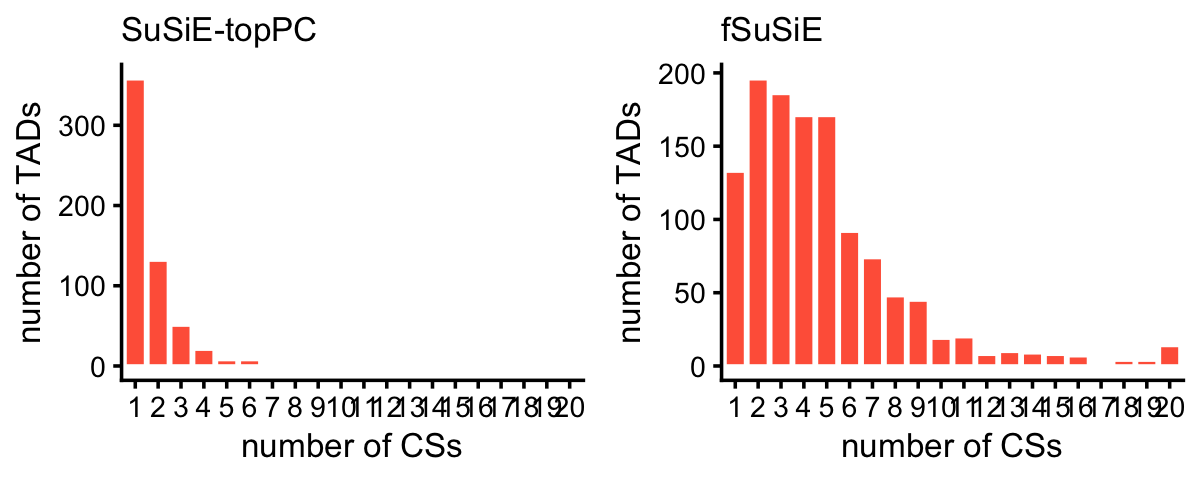
Compare discovery of causal SNPs (number of CSs) in the SuSiE-topPC and fSuSiE analyses:
dat1 <- get_cs_vs_tad_size(ha_snps_susie)
dat2 <- get_cs_vs_tad_size(ha_snps_fsusie)
dat1 <- dat1[c(1,3)]
dat2 <- dat2[c(1,3)]
names(dat1) <- c("tad","num_cs_susie")
names(dat2) <- c("tad","num_cs_fsusie")
dat <- merge(dat1,dat2,all = TRUE)
rows <- which(is.na(dat$num_cs_susie))
dat[rows,"num_cs_susie"] <- 0
pdat <- melt(with(dat,table(num_cs_susie,num_cs_fsusie)))
rows <- which(pdat$value == 0)
pdat[rows,"value"] <- NA
ggplot(pdat,aes(x = num_cs_susie,y = num_cs_fsusie,size = value)) +
  geom_point(color = "white",fill = "tomato",shape = 21) +
  geom_abline(intercept = 0,slope = 1,color = "black",linetype = "dotted") +
  scale_x_continuous(breaks = seq(0,20,2),limits = c(0,20)) +
  scale_y_continuous(breaks = seq(0,20,2),limits = c(0,20)) +
  scale_size(breaks = c(1,10,100)) +
  labs(x = "SuSiE-topPC",y = "fSuSiE",size = "number of TADs") +
  theme_cowplot(font_size = 10)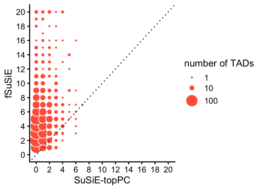
Compare the sizes of the CSs in the SuSiE-topPC and fSuSiE analyses:
bins <- c(0,1,2,5,10,20,Inf)
cs_size_susie  <- as.numeric(table(ha_snps_susie$cs))
cs_size_fsusie <- as.numeric(table(ha_snps_fsusie$cs))
cs_size_susie  <- cut(cs_size_susie,bins)
cs_size_fsusie <- cut(cs_size_fsusie,bins)
levels(cs_size_susie) <- bins[-1]
levels(cs_size_fsusie) <- bins[-1]
p1 <- ggplot(data.frame(cs_size = cs_size_susie),aes(x = cs_size)) +
  geom_histogram(stat = "count",color = "white",fill = "tomato",
                 width = 0.65) +
  labs(x = "CS size",y = "number of CSs",title = "SuSiE-topPC") +
  theme_cowplot(font_size = 10) +
  theme(plot.title = element_text(size = 10,face = "plain"))
p2 <- ggplot(data.frame(cs_size = cs_size_fsusie),aes(x = cs_size)) +
  geom_histogram(stat = "count",color = "white",fill = "tomato",
                 width = 0.65) +
  labs(x = "CS size",y = "number of CSs",title = "fSuSiE") +
  theme_cowplot(font_size = 10) +
  theme(plot.title = element_text(size = 10,face = "plain"))
plot_grid(p1,p2,nrow = 1,ncol = 2)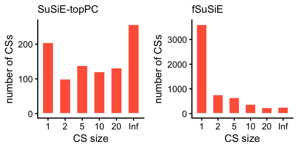
sessionInfo()
# R version 4.3.3 (2024-02-29)
# Platform: aarch64-apple-darwin20 (64-bit)
# Running under: macOS Sonoma 14.7.1
#
# Matrix products: default
# BLAS:   /Library/Frameworks/R.framework/Versions/4.3-arm64/Resources/lib/libRblas.0.dylib
# LAPACK: /Library/Frameworks/R.framework/Versions/4.3-arm64/Resources/lib/libRlapack.dylib;  LAPACK version 3.11.0
#
# locale:
# [1] en_US.UTF-8/en_US.UTF-8/en_US.UTF-8/C/en_US.UTF-8/en_US.UTF-8
#
# time zone: America/Chicago
# tzcode source: internal
#
# attached base packages:
# [1] stats     graphics  grDevices utils     datasets  methods   base
#
# other attached packages:
# [1] cowplot_1.1.3     ggplot2_3.5.0     data.table_1.15.2
#
# loaded via a namespace (and not attached):
#  [1] sass_0.4.9        utf8_1.2.4        generics_0.1.3    stringi_1.8.3
#  [5] digest_0.6.34     magrittr_2.0.3    evaluate_0.23     grid_4.3.3
#  [9] fastmap_1.1.1     plyr_1.8.9        R.oo_1.26.0       rprojroot_2.0.4
# [13] workflowr_1.7.1   jsonlite_1.8.8    R.utils_2.12.3    whisker_0.4.1
# [17] promises_1.2.1    fansi_1.0.6       scales_1.3.0      jquerylib_0.1.4
# [21] cli_3.6.4         rlang_1.1.5       R.methodsS3_1.8.2 munsell_0.5.0
# [25] withr_3.0.0       cachem_1.0.8      yaml_2.3.8        tools_4.3.3
# [29] reshape2_1.4.4    dplyr_1.1.4       colorspace_2.1-0  httpuv_1.6.14
# [33] vctrs_0.6.5       R6_2.5.1          lifecycle_1.0.4   git2r_0.33.0
# [37] stringr_1.5.1     fs_1.6.5          pkgconfig_2.0.3   pillar_1.9.0
# [41] bslib_0.6.1       later_1.3.2       gtable_0.3.4      glue_1.8.0
# [45] Rcpp_1.0.12       xfun_0.42         tibble_3.2.1      tidyselect_1.2.1
# [49] highr_0.10        knitr_1.45        farver_2.1.1      htmltools_0.5.8.1
# [53] rmarkdown_2.26    labeling_0.4.3    compiler_4.3.3