Examine ROSMAP RNA-seq and proteomics fine-mapping results
William Denault, Hao Sun, Angjing Liu, Peter Carbonetto, Gao Wang
Last updated: 2025-05-12
Checks: 7 0
Knit directory:
fsusie-experiments/analysis/
This reproducible R Markdown analysis was created with workflowr (version 1.7.1). The Checks tab describes the reproducibility checks that were applied when the results were created. The Past versions tab lists the development history.
Great! Since the R Markdown file has been committed to the Git repository, you know the exact version of the code that produced these results.
Great job! The global environment was empty. Objects defined in the global environment can affect the analysis in your R Markdown file in unknown ways. For reproduciblity it’s best to always run the code in an empty environment.
The command set.seed(1) was run prior to running the
code in the R Markdown file. Setting a seed ensures that any results
that rely on randomness, e.g. subsampling or permutations, are
reproducible.
Great job! Recording the operating system, R version, and package versions is critical for reproducibility.
Nice! There were no cached chunks for this analysis, so you can be confident that you successfully produced the results during this run.
Great job! Using relative paths to the files within your workflowr project makes it easier to run your code on other machines.
Great! You are using Git for version control. Tracking code development and connecting the code version to the results is critical for reproducibility.
The results in this page were generated with repository version 6c1c7c1. See the Past versions tab to see a history of the changes made to the R Markdown and HTML files.
Note that you need to be careful to ensure that all relevant files for
the analysis have been committed to Git prior to generating the results
(you can use wflow_publish or
wflow_git_commit). workflowr only checks the R Markdown
file, but you know if there are other scripts or data files that it
depends on. Below is the status of the Git repository when the results
were generated:
Untracked files:
    Untracked:  analysis/cs_sizes_protein.pdf
    Untracked:  analysis/cs_sizes_rnaseq.pdf
    Untracked:  analysis/rosmap_overview_cache/
    Untracked:  data/afreq.RData
    Untracked:  data/analysis_result/Fungen_xQTL.ENSG00000163808.cis_results_db.export.rds
    Untracked:  data/analysis_result/ROSMAP_haQTL.chr3_43915257_48413435.fsusie_mixture_normal_top_pc_weights.rds
    Untracked:  data/analysis_result/ROSMAP_mQTL.chr3_43915257_48413435.fsusie_mixture_normal_top_pc_weights.rds
    Untracked:  outputs/CASS4_all_effects.RData
    Untracked:  outputs/CASS4_obj.RData
    Untracked:  outputs/CD2AP_all_effects.RData
    Untracked:  outputs/CD2AP_obj.RData
    Untracked:  outputs/CR1_CR2_all_effects.RData
    Untracked:  outputs/CR1_CR2_obj.RData
    Untracked:  outputs/ROSMAP_DLPFC_mega_eQTL.cs_only.tsv.gz
    Untracked:  outputs/ROSMAP_DLPFC_pQTL.cs_only.tsv.gz
    Untracked:  outputs/ROSMAP_haQTL_cs_effect_ha_peak_annotation.tsv.gz
    Untracked:  outputs/ROSMAP_haQTL_cs_snp_annotation.tsv.gz
    Untracked:  outputs/ROSMAP_haQTL_cs_snp_toppc1_annotation.tsv.gz
    Untracked:  outputs/ROSMAP_haQTL_qtl_snp_qval0.05.tsv.gz
    Untracked:  outputs/ROSMAP_haQTL_qtl_snp_qval0.05_annotation.tsv.gz
    Untracked:  outputs/ROSMAP_mQTL_cs_effect_cpg_annotation.tsv.gz
    Untracked:  outputs/ROSMAP_mQTL_cs_snp_annotation.tsv.gz
    Untracked:  outputs/ROSMAP_mQTL_cs_snp_toppc1_annotation.tsv.gz
    Untracked:  outputs/ROSMAP_mQTL_qtl_snp_qval0.05.tsv.gz
    Untracked:  outputs/ROSMAP_mQTL_qtl_snp_qval0.05_annotation.tsv.gz
Note that any generated files, e.g. HTML, png, CSS, etc., are not included in this status report because it is ok for generated content to have uncommitted changes.
These are the previous versions of the repository in which changes were
made to the R Markdown (analysis/rosmap_rnaseq_protein.Rmd)
and HTML (docs/rosmap_rnaseq_protein.html) files. If you’ve
configured a remote Git repository (see ?wflow_git_remote),
click on the hyperlinks in the table below to view the files as they
were in that past version.
| File | Version | Author | Date | Message |
|---|---|---|---|---|
| Rmd | 6c1c7c1 | Peter Carbonetto | 2025-05-12 | workflowr::wflow_publish("rosmap_rnaseq_protein.Rmd", verbose = TRUE) |
| html | 4300655 | Peter Carbonetto | 2025-05-06 | Ran wflow_publish("rosmap_rnaseq_protein.Rmd"). |
| Rmd | 0f1725a | Peter Carbonetto | 2025-05-06 | Fixed code in rosmap_rnaseq_protein.Rmd to filter out eSNPs and pSNPS with MAF < 0.05. |
| html | aec2431 | Peter Carbonetto | 2025-05-06 | Added MAF filters to rosmap_rnaseq_protein analysis. |
| Rmd | a043de0 | Peter Carbonetto | 2025-05-06 | wflow_publish("rosmap_rnaseq_protein.Rmd", verbose = TRUE) |
| html | 9da7f17 | Peter Carbonetto | 2025-05-01 | A few small improvements to the histograms in the |
| Rmd | 94a3734 | Peter Carbonetto | 2025-05-01 | workflowr::wflow_publish("rosmap_rnaseq_protein.Rmd") |
| html | ad75894 | Peter Carbonetto | 2025-05-01 | Added histograms to the rosmap_rnaseq_protein analysis. |
| Rmd | 5a65993 | Peter Carbonetto | 2025-05-01 | workflowr::wflow_publish("rosmap_rnaseq_protein.Rmd") |
| Rmd | 1040101 | Peter Carbonetto | 2025-04-30 | Small edit to rosmap_rnaseq_protein.Rmd. |
| html | c8753a1 | Peter Carbonetto | 2025-04-30 | First build of the rosmap_rnaseq_protein analysis. |
| Rmd | 496ed0f | Peter Carbonetto | 2025-04-30 | wflow_publish("rosmap_rnaseq_protein.Rmd", verbose = TRUE, view = FALSE) |
| Rmd | 8a4d3fb | Peter Carbonetto | 2025-04-30 | workflowr::wflow_publish("index.Rmd") |
Note: If you would like to run this analysis on your computer, you will first need to download the fine-mapping outputs. They can be downloaded from here. Once you have downloaded the files, copy them to the “outputs” subdirectory.
Load a few packages used in the code below:
library(data.table)
library(ggplot2)
library(cowplot)
Load the RNA-seq fine-mapping results:
rnaseq <- fread("../outputs/ROSMAP_DLPFC_mega_eQTL.cs_only.tsv.gz",
                sep = "\t",header = TRUE,stringsAsFactors = FALSE)
class(rnaseq) <- "data.frame"
rnaseq <- rnaseq[c("gene","variant_id","chr","pos","ref","alt","maf",
                   "pip","cs_coverage_0.95_min_corr","context")]
rnaseq <-
  transform(rnaseq,
            gene = factor(gene),
            chr = factor(chr),
            ref = factor(ref),
            alt = factor(alt),
            cs_coverage_0.95_min_corr = factor(cs_coverage_0.95_min_corr),
            context = factor(context))
rnaseq <- subset(rnaseq,context == "DLPFC_DeJager_eQTL")
Note that, as discussed, we are using the “cs_coverage_0.95_min_corr” results, which applies a purity filter of 0.8 to the 95% CSs (the naming of this column does not make that clear).
Remove RNA expression SNPs (eSNPs) with MAF < 5%:
gene_cs <- with(rnaseq,paste(gene,cs_coverage_0.95_min_corr,sep = "_"))
gene_cs <- factor(gene_cs)
maf_cs  <- tapply(rnaseq,gene_cs,function (x) x$maf[which.max(x$pip)])
keep_cs <- names(which(maf_cs >= 0.05))
rows    <- is.element(gene_cs,keep_cs)
rnaseq  <- rnaseq[rows,]
Plot a histogram of the CS sizes for the RNA-seq fine-mapping:
bins <- c(0,1,2,5,10,20,Inf)
gene_cs <- with(rnaseq,paste(gene,cs_coverage_0.95_min_corr,sep = "_"))
gene_cs <- factor(gene_cs)
cs_size <- as.numeric(table(gene_cs))
cs_size <- cut(cs_size,bins)
levels(cs_size) <- bins[-1]
p <- ggplot(data.frame(cs_size = cs_size),aes(x = cs_size)) +
  geom_histogram(stat = "count",color = "white",fill = "dodgerblue",
                 width = 0.65) +
  labs(x = "CS size",y = "number of CSs") +
  theme_cowplot(font_size = 10)
print(p)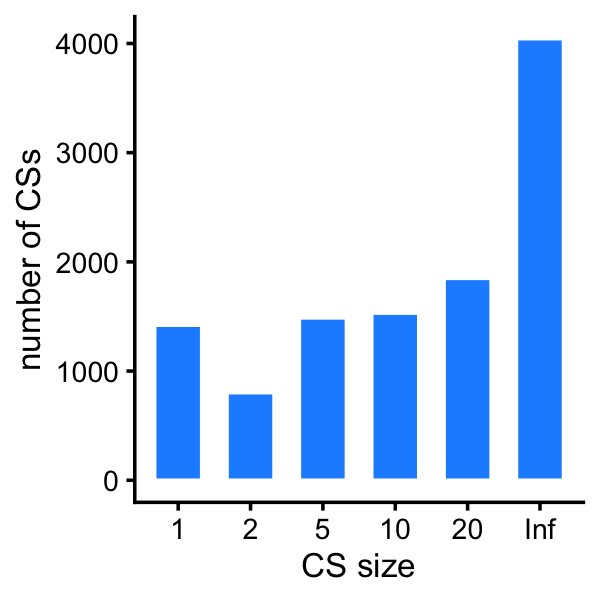
Here are the exact numbers:
table(cs_size)
# cs_size
#    1    2    5   10   20  Inf
# 1420  802 1487 1531 1849 4044
Load the protein fine-mapping results:
protein <- fread("../outputs/ROSMAP_DLPFC_pQTL.cs_only.tsv.gz",
                sep = "\t",header = TRUE,stringsAsFactors = FALSE)
class(protein) <- "data.frame"
protein <- protein[c("gene","variant_id","chr","pos","ref","alt","maf",
                     "pip","cs_coverage_0.95_min_corr","context")]
protein <-
  transform(protein,
            gene = factor(gene),
            chr = factor(chr),
            ref = factor(ref),
            alt = factor(alt),
            cs_coverage_0.95_min_corr = factor(cs_coverage_0.95_min_corr),
            context = factor(context))
protein <- subset(protein,context == "DLPFC_Bennett_pQTL")
Remove SNPs with MAF < 7.5%:
gene_cs <- with(protein,paste(gene,cs_coverage_0.95_min_corr,sep = "_"))
gene_cs <- factor(gene_cs)
maf_cs  <- tapply(protein,gene_cs,function (x) x$maf[which.max(x$pip)])
keep_cs <- names(which(maf_cs >= 0.05))
rows    <- is.element(gene_cs,keep_cs)
protein <- protein[rows,]
(Note that 7.5% to achieve a similar minor allele count threshold with the RNA-seq, methylation and H3K27ac data.)
Plot a histogram of the CS sizes for the proteomics fine-mapping:
gene_cs <- with(protein,paste(gene,cs_coverage_0.95_min_corr,sep = "_"))
gene_cs <- factor(gene_cs)
cs_size <- as.numeric(table(gene_cs))
cs_size <- cut(cs_size,bins)
levels(cs_size) <- bins[-1]
p <- ggplot(data.frame(cs_size = cs_size),aes(x = cs_size)) +
  geom_histogram(stat = "count",color = "white",fill = "darkorchid",
                 width = 0.65) +
  labs(x = "CS size",y = "number of CSs") +
  theme_cowplot(font_size = 10)
print(p)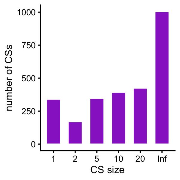
Here are the exact numbers:
table(cs_size)
# cs_size
#    1    2    5   10   20  Inf
#  340  170  347  393  424 1004
sessionInfo()
# R version 4.3.3 (2024-02-29)
# Platform: aarch64-apple-darwin20 (64-bit)
# Running under: macOS 15.4.1
#
# Matrix products: default
# BLAS:   /Library/Frameworks/R.framework/Versions/4.3-arm64/Resources/lib/libRblas.0.dylib
# LAPACK: /Library/Frameworks/R.framework/Versions/4.3-arm64/Resources/lib/libRlapack.dylib;  LAPACK version 3.11.0
#
# locale:
# [1] en_US.UTF-8/en_US.UTF-8/en_US.UTF-8/C/en_US.UTF-8/en_US.UTF-8
#
# time zone: America/Chicago
# tzcode source: internal
#
# attached base packages:
# [1] stats     graphics  grDevices utils     datasets  methods   base
#
# other attached packages:
# [1] cowplot_1.1.3     ggplot2_3.5.0     data.table_1.15.2
#
# loaded via a namespace (and not attached):
#  [1] sass_0.4.9        utf8_1.2.4        generics_0.1.3    stringi_1.8.3
#  [5] digest_0.6.34     magrittr_2.0.3    evaluate_1.0.3    grid_4.3.3
#  [9] fastmap_1.1.1     R.oo_1.26.0       rprojroot_2.0.4   workflowr_1.7.1
# [13] jsonlite_1.8.8    R.utils_2.12.3    whisker_0.4.1     promises_1.2.1
# [17] fansi_1.0.6       scales_1.3.0      textshaping_0.3.7 jquerylib_0.1.4
# [21] cli_3.6.4         rlang_1.1.5       R.methodsS3_1.8.2 munsell_0.5.0
# [25] withr_3.0.2       cachem_1.0.8      yaml_2.3.8        tools_4.3.3
# [29] dplyr_1.1.4       colorspace_2.1-0  httpuv_1.6.14     vctrs_0.6.5
# [33] R6_2.5.1          lifecycle_1.0.4   git2r_0.33.0      stringr_1.5.1
# [37] fs_1.6.5          ragg_1.2.7        pkgconfig_2.0.3   pillar_1.9.0
# [41] bslib_0.6.1       later_1.3.2       gtable_0.3.4      glue_1.8.0
# [45] Rcpp_1.0.12       systemfonts_1.0.6 xfun_0.42         tibble_3.2.1
# [49] tidyselect_1.2.1  highr_0.10        knitr_1.45        farver_2.1.1
# [53] htmltools_0.5.8.1 rmarkdown_2.26    labeling_0.4.3    compiler_4.3.3