Result3_SignalShape

Introduction

Signal setting
PVE
Packages / Libraries

Results

Source code

System Configuration

Last updated: 2019-10-19

Checks: 5 1

Knit directory: mr-ash-workflow/

This reproducible R Markdown analysis was created with workflowr (version 1.3.0). The Checks tab describes the reproducibility checks that were applied when the results were created. The Past versions tab lists the development history.

R Markdown file: uncommitted changes

The R Markdown file has unstaged changes. To know which version of the R Markdown file created these results, you’ll want to first commit it to the Git repo. If you’re still working on the analysis, you can ignore this warning. When you’re finished, you can run wflow_publish to commit the R Markdown file and build the HTML.

Environment: empty

Great job! The global environment was empty. Objects defined in the global environment can affect the analysis in your R Markdown file in unknown ways. For reproduciblity it’s best to always run the code in an empty environment.

Seed: set.seed(20191007)

The command set.seed(20191007) was run prior to running the code in the R Markdown file. Setting a seed ensures that any results that rely on randomness, e.g. subsampling or permutations, are reproducible.

Session information: recorded

Great job! Recording the operating system, R version, and package versions is critical for reproducibility.

Cache: none

Nice! There were no cached chunks for this analysis, so you can be confident that you successfully produced the results during this run.

Repository version: 92022af

Great! You are using Git for version control. Tracking code development and connecting the code version to the results is critical for reproducibility. The version displayed above was the version of the Git repository at the time these results were generated.

Note that you need to be careful to ensure that all relevant files for the analysis have been committed to Git prior to generating the results (you can use wflow_publish or wflow_git_commit). workflowr only checks the R Markdown file, but you know if there are other scripts or data files that it depends on. Below is the status of the Git repository when the results were generated:


Ignored files:
    Ignored:    .Rproj.user/

Untracked files:
    Untracked:  .DS_Store
    Untracked:  ETA_1_lambda.dat
    Untracked:  ETA_1_parBayesB.dat
    Untracked:  data/.DS_Store
    Untracked:  data/.Rapp.history
    Untracked:  mu.dat
    Untracked:  results/.Rapp.history
    Untracked:  results/changepoint1.RDS
    Untracked:  results/changepoint2.RDS
    Untracked:  results/realgenotype.RDS
    Untracked:  varE.dat

Unstaged changes:
    Modified:   analysis/Result2_Nonconvex.Rmd
    Modified:   analysis/Result6_PVE.Rmd
    Modified:   analysis/Result8_RealGenotype.Rmd
    Modified:   analysis/index.Rmd
    Modified:   code/method_wrapper.R
    Modified:   code/sim_wrapper.R
    Modified:   data/Thyroid.ENSG00000000971.RDS
    Modified:   data/Thyroid.ENSG00000031823.RDS

Note that any generated files, e.g. HTML, png, CSS, etc., are not included in this status report because it is ok for generated content to have uncommitted changes.

These are the previous versions of the R Markdown and HTML files. If you’ve configured a remote Git repository (see ?wflow_git_remote), click on the hyperlinks in the table below to view them.

File	Version	Author	Date	Message
html	79e1aab	Youngseok	2019-10-17	Build site.
html	fd5131c	Youngseok	2019-10-15	Build site.
html	70efed9	Youngseok	2019-10-14	Build site.
Rmd	6167c5a	Youngseok	2019-10-14	wflow_publish("analysis/*.Rmd")
html	bd36a79	Youngseok	2019-10-13	Build site.
Rmd	2368046	Youngseok	2019-10-13	wflow_publish("analysis/*.Rmd")

Introduction

Signal setting

We will use the following 6 different signal settings with the same sparsity $s = 20$ .

SparseLaplace: $\beta_j \sim \textrm{Laplace}(1)$ for $j \in J$ and $\beta_j = 0$ otherwise, where $J$ is a set of randomly $s$ indices in $\{1,\cdots,p\}$ , chosen uniformly at random.
SparseT2: $\beta_j \sim \textrm{t}_2$ for $j \in J$ and $\beta_j = 0$ otherwise, where $J$ is a set of randomly $s$ indices in $\{1,\cdots,p\}$ , chosen uniformly at random.
SparseT5: $\beta_j \sim \textrm{t}_5$ for $j \in J$ and $\beta_j = 0$ otherwise, where $J$ is a set of randomly $s$ indices in $\{1,\cdots,p\}$ , chosen uniformly at random.
SparseNormal: $\beta_j \sim N(0,\sigma_\beta^2)$ for $j \in J$ and $\beta_j = 0$ otherwise, where $J$ is a set of randomly $s$ indices in $\{1,\cdots,p\}$ , chosen uniformly at random.
SparseUniform: $\beta_j \sim \textrm{Unif}(0,1)$ for $j \in J$ and $\beta_j = 0$ otherwise, where $J$ is a set of randomly $s$ indices in $\{1,\cdots,p\}$ , chosen uniformly at random.
SparseConstant: $\beta_j = 1$ for $j \in J$ and $\beta_j = 0$ otherwise, where $J$ is a set of randomly $s$ indices in $\{1,\cdots,p\}$ , chosen uniformly at random.

The following is the tail behaviors of the above signal generating probability distributions.

library(ggplot2); library(cowplot)
x = seq(-100,100,0.01)
dat = rbind(data.frame(x = x, y = dexp(abs(x), 1, log = TRUE) / 2, signal = "SparseLaplace"),
            data.frame(x = x, y = dt(x, df = 2, log = TRUE), signal = "SparseT2"),
            data.frame(x = x, y = dt(x, df = 5, log = TRUE), signal = "SparseT5"),
            data.frame(x = x, y = dnorm(x, log = TRUE), signal = "SparseNormal"))
ggplot(dat) + geom_line(aes(x = x, y = y, color = signal)) + 
  coord_cartesian(ylim = c(-50,0)) + theme_cowplot(font_size = 14) +
  theme(axis.line    = element_blank()) +
  labs(x = "x", y = "logpdf(x)")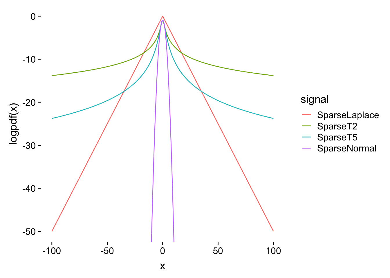

Version	Author	Date
bd36a79	Youngseok	2019-10-13

PVE

Packages / Libraries

A list of packages we have loaded is collapsed. Please click “code” to see the list.

library(Matrix); library(ggplot2); library(cowplot); library(susieR); library(BGLR);
library(glmnet); library(mr.ash); library(ncvreg); library(L0Learn); library(varbvs);
standardize = FALSE
source('code/method_wrapper.R')
source('code/sim_wrapper.R')

Results

res_df       = readRDS("results/signalshape_pve0.99.RDS")
method_list  = c("Mr.ASH","VarBVS","BayesB","Blasso","SuSiE","E-NET","Lasso","Ridge","SCAD","MCP","L0Learn")
method_level = c("Mr.ASH","E-NET","Lasso","Ridge",
                 "SCAD","MCP","L0Learn",
                 "VarBVS","BayesB","Blasso","SuSiE")
col          = gg_color_hue(11)
for (i in 1:6) {
res_df[[i]]$fit   = rep(method_list, each = 20)
res_df[[i]]$fit   = factor(res_df[[i]]$fit, levels =  c("Mr.ASH","E-NET","Lasso","Ridge",
                                            "SCAD","MCP","L0Learn",
                                            "VarBVS","BayesB","Blasso","SuSiE"))
some              = c(1,2,3,5,6,7)
res_df[[i]] = res_df[[i]][res_df[[i]]$fit %in% method_level[some],]
}
pp = list()
signal_name = c("SparseLaplace","SparseT2","SparseT5","SparseNormal","SparseUnif","SparseConst")
for (i in 1:6) {
  d       = res_df[[i]]
  pp[[i]] = my.box(d, "fit", "pred", values = col[some]) +
  theme(axis.line    = element_blank(),
        axis.text.x  = element_text(angle = 45,hjust = 1),
        legend.position = "none") +
  geom_hline(yintercept = median(d$pred[d$fit == "Mr.ASH"]), col = col[1],
             linetype = "dotted", size = 1.5) +
  scale_y_continuous(trans = "log10", breaks = c(1,1.2,1.4,1.6,1.8,2.0)) +
  coord_cartesian(ylim = c(0.95,1.8))
  subtitle  = ggdraw() + draw_label(paste(paste("Signal: ",signal_name[i], sep = ""),"", sep = ""),
                                    fontface  = 'bold', size = 18)
  pp[[i]]   = plot_grid(subtitle, pp[[i]], ncol = 1, rel_heights = c(0.06,0.95))
}
fig_main  = plot_grid(pp[[1]],pp[[2]],pp[[3]],pp[[4]],pp[[5]],pp[[6]], nrow = 2, rel_widths = c(0.3,0.3,0.3,0.3))
title     = ggdraw() + draw_label("Prediction Error (log-scale)", fontface = 'bold', size = 20) 
subtitle  = ggdraw() + draw_label("Scenario: LowdimIndepGauss, n = 500, p = 2000, s = 20, pve = 0.99", fontface = 'bold', size = 18)
fig       = plot_grid(title,subtitle,fig_main, ncol = 1, rel_heights = c(0.04,0.06,0.95))
fig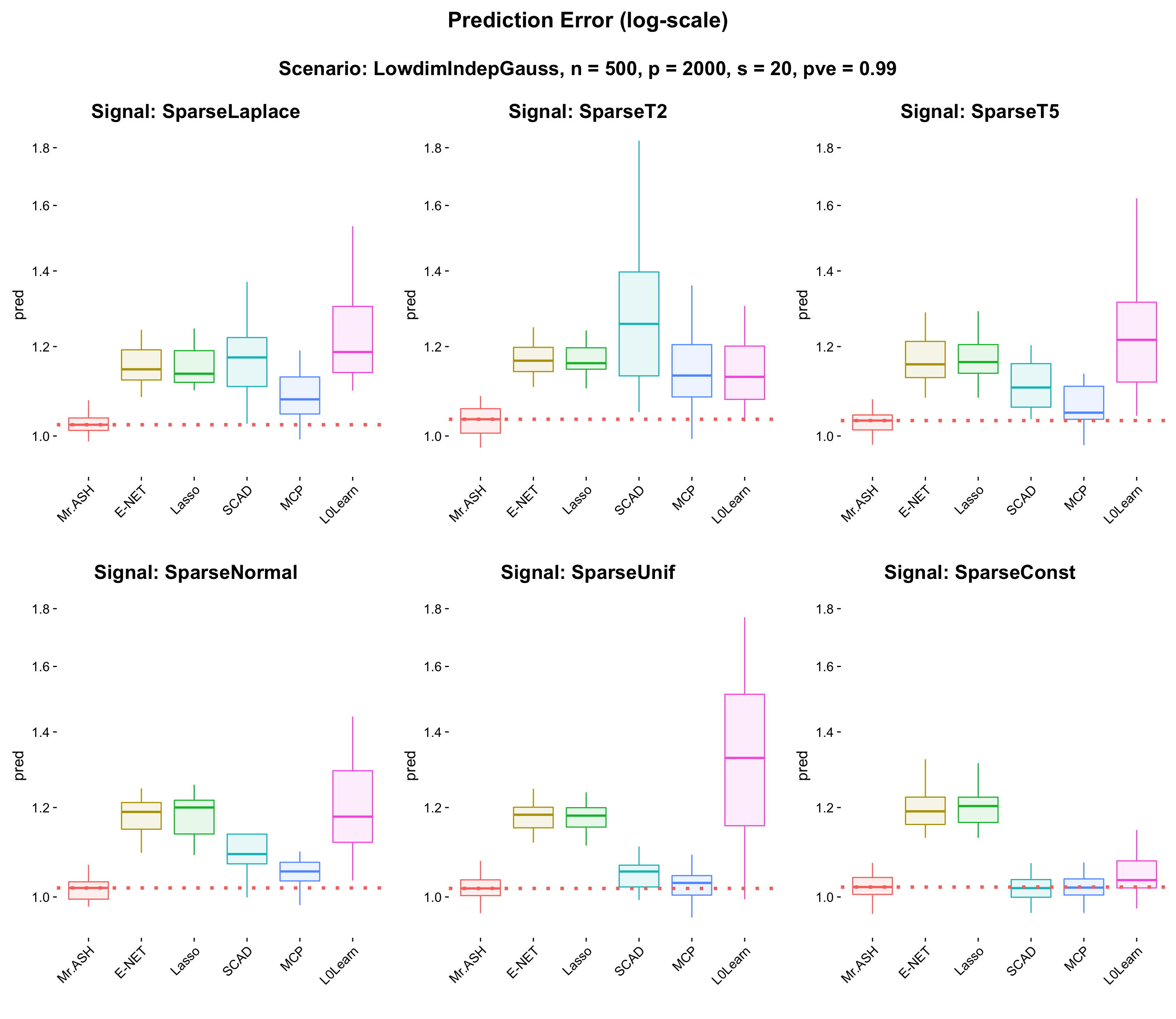

Version	Author	Date
bd36a79	Youngseok	2019-10-13

sdat = rbind(res_df[[1]], res_df[[2]], res_df[[3]], res_df[[4]], res_df[[5]], res_df[[6]])
p1       = my.box(res_df[[1]], "fit", "time", values = gg_color_hue(11)[c(1,3,7,6,9,11,2,4,5,8)]) +
  theme(axis.line    = element_blank(),
        axis.text.x  = element_text(angle = 45,hjust = 1),
        legend.position = "none") +
  scale_y_continuous(trans = "log10")
p0        = ggplot() + geom_blank() + theme_cowplot() + theme(axis.line = element_blank())
fig_main  = plot_grid(p0,p1,p0, nrow = 1, rel_widths = c(0.6,0.6,0.6))
title     = ggdraw() + draw_label("Computation time (log-scale)", fontface = 'bold', size = 20) 
subtitle  = ggdraw() + draw_label("Scenario: IndepGauss + SparseSignals, n = 500, p = 2000, s = 20, pve = 0.99", fontface  = 'bold', size = 18) 
fig       = plot_grid(title,subtitle,fig_main, ncol = 1, rel_heights = c(0.1,0.06,0.95))
fig

Version	Author	Date
bd36a79	Youngseok	2019-10-13

Source code

The source code will be popped up when you click code on the right side.

tdat1        = list()
n            = 500
p            = 2000
s            = 20
signal_list  = c("lap","t2","t5","normal","unif","const")
method_list  = c("varbvs","bayesb","blasso","susie","enet","lasso","ridge","scad","mcp","l0learn")
method_num   = length(method_list) + 1
iter_num     = 20
pred         = matrix(0, iter_num, method_num); colnames(pred) = c("mr.ash", method_list)
time         = matrix(0, iter_num, method_num); colnames(time) = c("mr.ash", method_list)

for (iter in 1:6) {
for (i in 1:20) {
  data          = simulate_data(n, p, s = s, seed = i, signal = signal_list[iter], pve = 0.99)


 
  for (j in 1:length(method_list)) {
    fit.method    = get(paste("fit.",method_list[j],sep = ""))
    fit           = fit.method(data$X, data$y, data$X.test, data$y.test, seed = i)
    pred[i,j+1]   = fit$rsse / data$sigma / sqrt(n)
    time[i,j+1]   = fit$t
  }
 
  fit         = fit.mr.ash(data$X, data$y, data$X.test, data$y.test, seed = i,
                           sa2 = (2^((0:19) / 5 / sqrt(2)^(iter-1)) - 1)^2)
  pred[i,1]   = fit$rsse / data$sigma / sqrt(n)
  time[i,1]   = fit$t
}
}
tdat1[[iter]] = data.frame(pred = c(pred), time = c(time), fit = rep(c("mr.ash", method_list), each = 20))

System Configuration

Click the below Session Info.

sessionInfo()

R version 3.5.3 (2019-03-11)
Platform: x86_64-apple-darwin15.6.0 (64-bit)
Running under: macOS High Sierra 10.13.3

Matrix products: default
BLAS: /Library/Frameworks/R.framework/Versions/3.5/Resources/lib/libRblas.0.dylib
LAPACK: /Library/Frameworks/R.framework/Versions/3.5/Resources/lib/libRlapack.dylib

locale:
[1] en_US.UTF-8/en_US.UTF-8/en_US.UTF-8/C/en_US.UTF-8/en_US.UTF-8

attached base packages:
[1] stats     graphics  grDevices utils     datasets  methods   base     

other attached packages:
 [1] varbvs_2.6-5  L0Learn_1.1.0 ncvreg_3.11-1 mr.ash_0.1-2  glmnet_2.0-16
 [6] foreach_1.4.4 BGLR_1.0.8    susieR_0.7.1  Matrix_1.2-17 cowplot_0.9.4
[11] ggplot2_3.2.1

loaded via a namespace (and not attached):
 [1] Rcpp_1.0.2          RColorBrewer_1.1-2  plyr_1.8.4         
 [4] pillar_1.3.1        compiler_3.5.3      git2r_0.25.2       
 [7] workflowr_1.3.0     iterators_1.0.10    tools_3.5.3        
[10] digest_0.6.18       evaluate_0.13       tibble_2.1.1       
[13] gtable_0.3.0        lattice_0.20-38     pkgconfig_2.0.2    
[16] rlang_0.4.0         yaml_2.2.0          xfun_0.6           
[19] withr_2.1.2         stringr_1.4.0       dplyr_0.8.3        
[22] knitr_1.22          fs_1.3.0            rprojroot_1.3-2    
[25] grid_3.5.3          tidyselect_0.2.5    glue_1.3.1         
[28] R6_2.4.0            rmarkdown_1.12      latticeExtra_0.6-28
[31] reshape2_1.4.3      purrr_0.3.2         magrittr_1.5       
[34] whisker_0.3-2       codetools_0.2-16    backports_1.1.4    
[37] scales_1.0.0        htmltools_0.4.0     assertthat_0.2.1   
[40] colorspace_1.4-1    labeling_0.3        nor1mix_1.2-3      
[43] stringi_1.4.3       lazyeval_0.2.2      munsell_0.5.0      
[46] truncnorm_1.0-8     crayon_1.3.4