Result1_Ridge

Introduction

Design setting
Signal setting
PVE
Performance Measure

Methods

Optimal Ridge
Elastic Net
Other methods
Packages / Libraries

Results

Source code

System Configuration

Last updated: 2019-10-21

Checks: 7 0

Knit directory: mr-ash-workflow/

This reproducible R Markdown analysis was created with workflowr (version 1.4.0). The Checks tab describes the reproducibility checks that were applied when the results were created. The Past versions tab lists the development history.

R Markdown file: up-to-date

Great! Since the R Markdown file has been committed to the Git repository, you know the exact version of the code that produced these results.

Environment: empty

Great job! The global environment was empty. Objects defined in the global environment can affect the analysis in your R Markdown file in unknown ways. For reproduciblity it’s best to always run the code in an empty environment.

Seed: set.seed(20191007)

The command set.seed(20191007) was run prior to running the code in the R Markdown file. Setting a seed ensures that any results that rely on randomness, e.g. subsampling or permutations, are reproducible.

Session information: recorded

Great job! Recording the operating system, R version, and package versions is critical for reproducibility.

Cache: none

Nice! There were no cached chunks for this analysis, so you can be confident that you successfully produced the results during this run.

File paths: relative

Great job! Using relative paths to the files within your workflowr project makes it easier to run your code on other machines.

Repository version: 506cf21

Great! You are using Git for version control. Tracking code development and connecting the code version to the results is critical for reproducibility. The version displayed above was the version of the Git repository at the time these results were generated.

Note that you need to be careful to ensure that all relevant files for the analysis have been committed to Git prior to generating the results (you can use wflow_publish or wflow_git_commit). workflowr only checks the R Markdown file, but you know if there are other scripts or data files that it depends on. Below is the status of the Git repository when the results were generated:


Ignored files:
    Ignored:    .Rhistory
    Ignored:    .Rproj.user/
    Ignored:    analysis/ETA_1_lambda.dat
    Ignored:    analysis/ETA_1_parBayesB.dat
    Ignored:    analysis/mu.dat
    Ignored:    analysis/varE.dat

Untracked files:
    Untracked:  .DS_Store
    Untracked:  .Rapp.history
    Untracked:  docs/figure/Result9_Changepoint.Rmd/
    Untracked:  results/estsigma.RDS

Note that any generated files, e.g. HTML, png, CSS, etc., are not included in this status report because it is ok for generated content to have uncommitted changes.

These are the previous versions of the R Markdown and HTML files. If you’ve configured a remote Git repository (see ?wflow_git_remote), click on the hyperlinks in the table below to view them.

File	Version	Author	Date	Message
Rmd	585044e	Youngseok Kim	2019-10-21	update
html	79e1aab	Youngseok	2019-10-17	Build site.
html	fd5131c	Youngseok	2019-10-15	Build site.
html	e365595	Youngseok	2019-10-14	Build site.
Rmd	9f05c82	Youngseok	2019-10-14	wflow_publish(“analysis/Result1_Ridge.Rmd”)
html	70efed9	Youngseok	2019-10-14	Build site.
html	bd36a79	Youngseok	2019-10-14	Build site.
Rmd	2368046	Youngseok	2019-10-14	wflow_publish("analysis/*.Rmd")

Introduction

This .Rmd file is to plot results for the experiment MR.ASH versus Elastic Net (E-NET). However, for the comprehensive comparison, we also include results from all the other methods.

glmnet R package: Ridge, Lasso, E-NET
ncvreg R package: SCAD, MCP
L0Learn R package: L0Learn
BGLR R package: BayesB, Blasso (Bayesian Lasso)
susieR R package: SuSiE (Sum of Single Effect)
varbvs R package: VarBVS (Variational Bayes Variable Selection)

The experiment is based on the following simulation setting.

Design setting

We sample the standard i.i.d. Gaussian measurement $X_{ij} \sim N(0,1)$ anda construct $X \in \mathbb{R}^p$ with $n = 500$ and $p \in \{50,100,200,500,1000,2000\}$ .

Signal setting

We sample the i.i.d. normal coefficients $\beta_j \sim N(0,\sigma_\beta^2)$ for $j = 1,\cdots,p$ , or $\beta \sim N(0,\sigma_\beta^2 I_p)$ .

This signal will be called normal.

PVE

Then we sample $y = X\beta + \epsilon$ , where $\epsilon \sim N(0,\sigma^2 I_n)$ .

We fix PVE = 0.5, where PVE is the proportion of variance explained, defined by

${\rm PVE} = \frac{\textrm{Var}(X\beta)}{\textrm{Var}(X\beta) + \sigma^2},$ where $\textrm{Var}(a)$ denotes the sample variance of $a$ calculated using R function var. To this end, we set $\sigma^2 = \textrm{Var}(X\beta)$ .

Performance Measure

The above two figures display the prediction error. The prediction error we define here is

$\textrm{Pred.Err}(\hat\beta;y_{\rm test}, X_{\rm test}) = \frac{\textrm{RMSE}}{\sigma} = \frac{\|y_{\rm test} - X_{\rm test} \hat\beta \|}{\sqrt{n}\sigma}$ where $y_{\rm test}$ and $X_{\rm test}$ are test data sample in the same way. If $\hat\beta$ is fairly accurate, then we expect that $\rm RMSE$ is similar to $\sigma$ . Therefore in average $\textrm{Pred.Err} \geq 1$ and the smaller the better.

Methods

In what follows, we briefly describe the comparison methods.

Optimal Ridge

Let us recall that we sample the i.i.d. normal coefficients $\beta_j \sim N(0,\sigma_\beta^2)$ for $j = 1,\cdots,p$ , or $\beta \sim N(0,\sigma_\beta^2 I_p)$ .

We expect that in this simulation setting, the ridge regression with the optimal tuning parameter $\lambda$ will perform the best.

$p(\beta|y,X,\sigma^2) \propto p(y|X,\beta,\sigma^2) p(\beta) \propto \exp\left( - \frac{1}{2\sigma^2} \|y - X\beta\|_2^2 - \frac{1}{2\sigma_\beta^2} \|\beta\|_2^2 \right)$

This implies that $p(\beta|y,X,\sigma^2)$ is again a multivariate normal distribution and thus the posterior mode is equal to the posterior mean. Thus the optimal $\lambda$ is $\sigma^2 / (n\sigma_\beta^2)$ .

Elastic Net

The glmnet R package provides an elastic net implementation. It seeks to minimize the following objective function.

$\frac{1}{2n} \| y - X\beta \|^2 + \lambda \left(\alpha \|\beta\|_1 + 0.5 (1 - \alpha) \|\beta\|_2^2 \right)$

$\lambda$ and $\alpha$ are tuning parameters. For a fixed $\alpha$ in $\{ 0.1 * (a-1) : a = 1,\cdots, 11$ , we run cv.glmnet with the default setting to tune $\lambda$ by cross-validation. Then we select a best tuple of $\alpha$ and $\lambda$ that minimizes the cross-validation error.

Other methods

We also compare other methods implemented in R. The list of packages and methods is provided below.

ncvreg R package: SCAD, MCP
L0Learn R package: L0Learn
BGLR R package: BayesB, Blasso (Bayesian Lasso)
susieR R package: SuSiE (Sum of Single Effect)
varbvs R package: VarBVS (Variational Bayes Variable Selection)

Packages / Libraries

A list of packages we have loaded is collapsed. Please click “code” to see the list.

library(Matrix); library(ggplot2); library(cowplot); library(susieR); library(BGLR);
library(glmnet); library(varbvs2); library(ncvreg); library(L0Learn); library(varbvs);
standardize = FALSE
source('code/method_wrapper.R')
source('code/sim_wrapper.R')

Results

The result is summarized below.

res_df       = readRDS("results/ridge_pve0.5.RDS")
p_list       = c(50,100,200,500,1000,2000)
method_list  = c("Mr.ASH","VarBVS","BayesB","Blasso","SuSiE","E-NET","Lasso","Ridge","SCAD","MCP","L0Learn","Ridge.opt")
col          = gg_color_hue(11)
sdat = data.frame()
for (i in 1:6) {
  sdat       = rbind(sdat, data.frame(pred = colMeans(matrix(res_df[[i]]$pred,20,12)),
                                      time = colMeans(matrix(res_df[[i]]$time,20,12)),
                                      p = p_list[i],
                                      fit = method_list))
}
sdat$fit    = factor(sdat$fit, levels =  c("Mr.ASH","E-NET","Lasso","Ridge",
                                           "SCAD","MCP","L0Learn",
                                           "VarBVS","BayesB","Blasso","SuSiE",
                                           "Ridge.opt"))
sdat1       = sdat[sdat$fit %in% c("Mr.ASH","E-NET","Lasso","Ridge","Ridge.opt"),]
sdat2       = sdat[sdat$fit %in% c("Mr.ASH","E-NET","SCAD","MCP","L0Learn","Ridge.opt"),]
sdat3       = sdat[sdat$fit %in% c("Mr.ASH","VarBVS","BayesB","Blasso","SuSiE","Ridge.opt"),]

p1 = ggplot(sdat1) + geom_line(aes(x = p, y = pred, color = fit)) +
  geom_point(aes(x = p, y = pred, color = fit, shape = fit), size = 2.5) +
  theme_cowplot(font_size = 14) +
  scale_x_continuous(trans = "log10", breaks = p_list) +
  labs(y = "predictior error (rmse / sigma)", x = "number of coefficients (p)") +
  theme(axis.line = element_blank(),
        plot.title = element_text(hjust = 0.5)) +
  scale_color_manual(values = c(col[c(1,2,3,4)],"gray50")) +
  scale_shape_manual(values = c(19,17,24,25,15)) +
  scale_y_continuous(trans = "log10", limits = c(1.04,1.46), breaks = c(1.1,1.2,1.3,1.4))
p2 = ggplot(sdat2) + geom_line(aes(x = p, y = pred, color = fit)) +
  geom_point(aes(x = p, y = pred, color = fit, shape = fit), size = 2.5) +
  theme_cowplot(font_size = 14) +
  scale_x_continuous(trans = "log10", breaks = p_list) +
  labs(y = "", x = "number of coefficients (p)") +
  theme(axis.line = element_blank(),
        plot.title = element_text(hjust = 0.5)) +
  scale_color_manual(values = c(col[c(1,2,5,6,7)],"gray50")) +
  scale_shape_manual(values = c(19,17,9,3,11,15)) +
  scale_y_continuous(trans = "log10", limits = c(1.04,1.46), breaks = c(1.1,1.2,1.3,1.4))
p3 = ggplot(sdat3) + geom_line(aes(x = p, y = pred, color = fit)) +
  geom_point(aes(x = p, y = pred, color = fit, shape = fit), size = 2.5) +
  theme_cowplot(font_size = 14) +
  scale_x_continuous(trans = "log10", breaks = p_list) +
  labs(y = "", x = "number of coefficients (p)") +
  theme(axis.line = element_blank(),
        plot.title = element_text(hjust = 0.5)) +
  scale_color_manual(values = c(col[c(1,8,9,10,11)],"gray50")) +
  scale_shape_manual(values = c(19,4,5,7,8,15)) +
  scale_y_continuous(trans = "log10", limits = c(1.04,1.46), breaks = c(1.1,1.2,1.3,1.4))
fig_main  = plot_grid(p1,p2,p3, nrow = 1, rel_widths = c(0.35,0.35,0.3))
title     = ggdraw() + draw_label("Prediction Error (log-scale)", fontface = 'bold', size = 20) 
subtitle  = ggdraw() + draw_label("Scenario: IndepGauss + Normal, n = 500, p = 50,100,200,500,1000,2000, pve = 0.5", fontface  = 'bold', size = 18) 
fig       = plot_grid(title,subtitle,fig_main, ncol = 1, rel_heights = c(0.1,0.06,0.95))
fig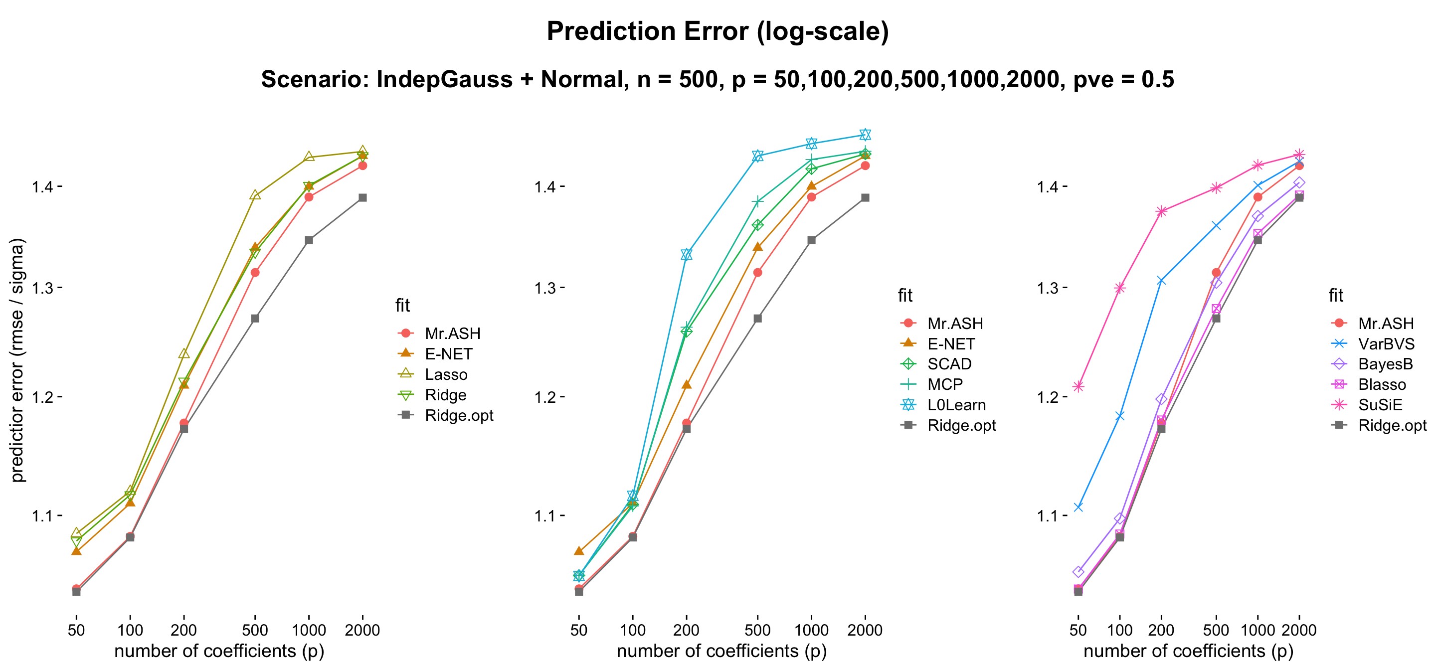

Version	Author	Date
bd36a79	Youngseok	2019-10-14

p4  = my.box(sdat[sdat$fit != "Ridge.opt",], "fit", "time",
             gg_color_hue(11)) +
  theme(axis.line    = element_blank(),
        axis.text.x  = element_text(angle = 45,hjust = 1),
        legend.position = "none") +
  scale_y_continuous(trans = "log10")
title     = ggdraw() + draw_label("Computation time (log-scale)", fontface = 'bold', size = 20) 
subtitle  = ggdraw() + draw_label("Scenario: IndepGauss + Normal, n = 500, p = 50,100,200,500,1000,2000, pve = 0.5", fontface  = 'bold', size = 18) 
p0        = ggplot() + geom_blank() + theme_cowplot() + theme(axis.line = element_blank())
fig_main  = plot_grid(p0,p4,p0, nrow = 1, rel_widths = c(0.3,0.6,0.3))
fig       = plot_grid(title,subtitle,fig_main, ncol = 1, rel_heights = c(0.1,0.06,0.95))
fig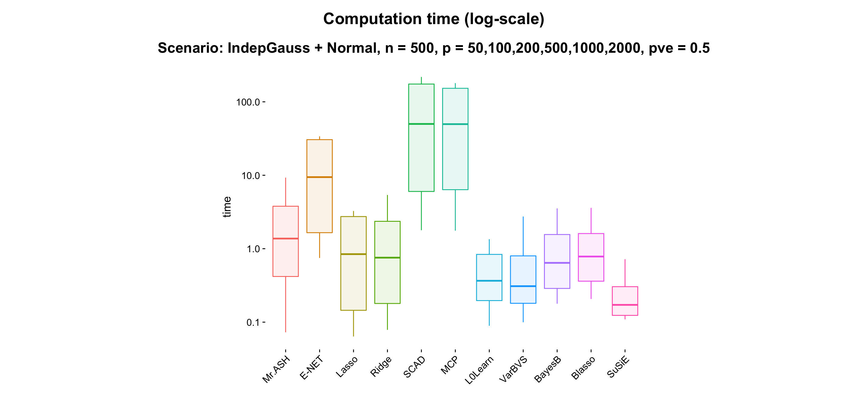

Version	Author	Date
bd36a79	Youngseok	2019-10-14

Source code

The source code will be popped up when you click code on the right side.

setwd("..")
library(Matrix); library(ggplot2); library(cowplot); library(susieR); library(BGLR);
library(glmnet); library(mr.ash); library(ncvreg); library(L0Learn); library(varbvs);
standardize = FALSE
source('code/method_wrapper.R')
source('code/sim_wrapper.R')
tdat1        = list()
n            = 500
p_range      = c(50,100,200,500,1000,2000)
method_list  = c("varbvs","bayesb","blasso","susie","enet","lasso","ridge","scad","mcp","l0learn")
method_list2 = c("mr.ash", method_list, "mr.ash.order", "mr.ash.init", "ridge.opt")
method_num   = length(method_list) + 4
iter_num     = 20
pred         = matrix(0, iter_num, method_num);
time         = matrix(0, iter_num, method_num);
colnames(pred) <- colnames(time) <- method_list2

for (iter in 1:6) {
p               = p_range[iter]
for (i in 1:20) {
  data          = simulate_data(n, p, s = p, seed = i, signal = "normal", pve = 0.5)
 
  for (j in 1:length(method_list)) {
    fit.method    = get(paste("fit.",method_list[j],sep = ""))
    fit           = fit.method(data$X, data$y, data$X.test, data$y.test, seed = i)
    pred[i,j+1]   = fit$rsse / data$sigma / sqrt(n)
    time[i,j+1]   = fit$t
    
    if (method_list[j] == "lasso") {
      lasso.path.order = mr.ash:::path.order(fit$fit$glmnet.fit)
      lasso.beta       = as.vector(coef(fit$fit))[-1]
      lasso.time       = c(fit$t, fit$t2)
    }
  }
 
  fit         = fit.mr.ash(data$X, data$y, data$X.test, data$y.test, seed = i,
                           sa2 = (2^((0:19) / 5 / 2^iter) - 1)^2)
  pred[i,1]   = fit$rsse / data$sigma / sqrt(n)
  time[i,1]   = fit$t
  
  fit         = fit.mr.ash2(data$X, data$y, data$X.test, data$y.test, seed = i,
                            update.order = lasso.path.order,
                            sa2 = (2^((0:19) / 5) - 1)^2)
  pred[i,j+2] = fit$rsse / data$sigma / sqrt(n)
  time[i,j+2] = fit$t + lasso.time[2]
  
  fit         = fit.mr.ash2(data$X, data$y, data$X.test, data$y.test, seed = i,
                            beta.init = lasso.beta,
                            sa2 = (2^((0:19) / 5) - 1)^2)
  pred[i,j+3] = fit$rsse / data$sigma / sqrt(n)
  time[i,j+3] = fit$t + lasso.time[1]
  
  fit         = fit.ridge.opt(data$X, data$y, data$X.test, data$y.test, data$sigma, seed = i)
  pred[i,method_num] = fit$rsse / data$sigma / sqrt(n)
  time[i,method_num] = -Inf
  cat(i," ")
}
cat("\n")
print(c(colMeans(pred)))
tdat1[[iter]] = data.frame(pred = c(pred), time = c(time),
                           fit = rep(method_list2, each = 20))
}

System Configuration

Click the below Session Info.

sessionInfo()

R version 3.5.3 (2019-03-11)
Platform: x86_64-apple-darwin15.6.0 (64-bit)
Running under: macOS Mojave 10.14

Matrix products: default
BLAS: /Library/Frameworks/R.framework/Versions/3.5/Resources/lib/libRblas.0.dylib
LAPACK: /Library/Frameworks/R.framework/Versions/3.5/Resources/lib/libRlapack.dylib

locale:
[1] en_US.UTF-8/en_US.UTF-8/en_US.UTF-8/C/en_US.UTF-8/en_US.UTF-8

attached base packages:
[1] stats     graphics  grDevices utils     datasets  methods   base     

other attached packages:
 [1] varbvs_2.5-16 L0Learn_1.2.0 ncvreg_3.11-1 varbvs2_0.1-1 glmnet_2.0-18
 [6] foreach_1.4.7 BGLR_1.0.8    susieR_0.8.0  cowplot_1.0.0 ggplot2_3.2.1
[11] Matrix_1.2-17

loaded via a namespace (and not attached):
 [1] Rcpp_1.0.2          RColorBrewer_1.1-2  plyr_1.8.4         
 [4] compiler_3.5.3      pillar_1.4.2        git2r_0.26.1       
 [7] workflowr_1.4.0     iterators_1.0.12    tools_3.5.3        
[10] digest_0.6.21       evaluate_0.14       tibble_2.1.3       
[13] gtable_0.3.0        lattice_0.20-38     pkgconfig_2.0.3    
[16] rlang_0.4.0         yaml_2.2.0          xfun_0.9           
[19] withr_2.1.2         stringr_1.4.0       dplyr_0.8.3        
[22] knitr_1.25          fs_1.3.1            rprojroot_1.3-2    
[25] grid_3.5.3          tidyselect_0.2.5    glue_1.3.1         
[28] R6_2.4.0            rmarkdown_1.15      latticeExtra_0.6-28
[31] reshape2_1.4.3      purrr_0.3.2         magrittr_1.5       
[34] whisker_0.4         codetools_0.2-16    backports_1.1.4    
[37] scales_1.0.0        htmltools_0.3.6     assertthat_0.2.1   
[40] colorspace_1.4-1    nor1mix_1.3-0       stringi_1.4.3      
[43] lazyeval_0.2.2      munsell_0.5.0       truncnorm_1.0-8    
[46] crayon_1.3.4