Result1_Ridge
Last updated: 2019-10-22
Checks: 6 0
Knit directory: mr-ash-workflow/
This reproducible R Markdown analysis was created with workflowr (version 1.3.0). The Checks tab describes the reproducibility checks that were applied when the results were created. The Past versions tab lists the development history.
Great! Since the R Markdown file has been committed to the Git repository, you know the exact version of the code that produced these results.
Great job! The global environment was empty. Objects defined in the global environment can affect the analysis in your R Markdown file in unknown ways. For reproduciblity it’s best to always run the code in an empty environment.
The command set.seed(20191007) was run prior to running the code in the R Markdown file. Setting a seed ensures that any results that rely on randomness, e.g. subsampling or permutations, are reproducible.
Great job! Recording the operating system, R version, and package versions is critical for reproducibility.
Nice! There were no cached chunks for this analysis, so you can be confident that you successfully produced the results during this run.
Great! You are using Git for version control. Tracking code development and connecting the code version to the results is critical for reproducibility. The version displayed above was the version of the Git repository at the time these results were generated.
Note that you need to be careful to ensure that all relevant files for the analysis have been committed to Git prior to generating the results (you can use wflow_publish or wflow_git_commit). workflowr only checks the R Markdown file, but you know if there are other scripts or data files that it depends on. Below is the status of the Git repository when the results were generated:
Ignored files:
    Ignored:    .Rhistory
    Ignored:    .Rproj.user/
    Ignored:    ETA_1_lambda.dat
    Ignored:    ETA_1_parBayesB.dat
    Ignored:    analysis/ETA_1_lambda.dat
    Ignored:    analysis/ETA_1_parBayesB.dat
    Ignored:    analysis/mu.dat
    Ignored:    analysis/varE.dat
    Ignored:    mu.dat
    Ignored:    varE.dat

Untracked files:
    Untracked:  .DS_Store
    Untracked:  results/equicorr.RDS
    Untracked:  results/localcorr.RDS
    Untracked:  results/localcorr.REDS

Unstaged changes:
    Modified:   analysis/Result4_Highdim.Rmd
    Modified:   analysis/index.Rmd
    Modified:   code/sim_wrapper.R
Note that any generated files, e.g. HTML, png, CSS, etc., are not included in this status report because it is ok for generated content to have uncommitted changes.
These are the previous versions of the R Markdown and HTML files. If you’ve configured a remote Git repository (see ?wflow_git_remote), click on the hyperlinks in the table below to view them.
| File | Version | Author | Date | Message |
|---|---|---|---|---|
| Rmd | c3d30a8 | Youngseok Kim | 2019-10-22 | wflow_publish(“analysis/Result1_Ridge.Rmd”) |
| html | 2443c8b | Youngseok Kim | 2019-10-22 | Build site. |
| Rmd | 8e7e970 | Youngseok Kim | 2019-10-22 | wflow_publish(“analysis/Result1_Ridge.Rmd”) |
| Rmd | e35b458 | Youngseok | 2019-10-22 | update gitignore |
| Rmd | 4f8651a | Youngseok | 2019-10-22 | update changepoint analysis |
| html | 7d6c1c8 | Youngseok | 2019-10-21 | Build site. |
| Rmd | 585044e | Youngseok Kim | 2019-10-21 | update |
| html | 79e1aab | Youngseok | 2019-10-17 | Build site. |
| html | fd5131c | Youngseok | 2019-10-15 | Build site. |
| html | e365595 | Youngseok | 2019-10-14 | Build site. |
| Rmd | 9f05c82 | Youngseok | 2019-10-14 | wflow_publish(“analysis/Result1_Ridge.Rmd”) |
| html | 70efed9 | Youngseok | 2019-10-14 | Build site. |
| html | bd36a79 | Youngseok | 2019-10-13 | Build site. |
| Rmd | 2368046 | Youngseok | 2019-10-13 | wflow_publish("analysis/*.Rmd") |
Introduction
The experiment is based on the following simulation setting.
Design setting
We sample the standard i.i.d. Gaussian measurement \(X_{ij} \sim N(0,1)\) anda construct \(X \in \mathbb{R}^p\) with \(n = 500\) and \(p \in \{50,100,200,500,1000,2000\}\).
Signal setting
We sample the i.i.d. normal coefficients \(\beta_j \sim N(0,\sigma_\beta^2)\) for \(j = 1,\cdots,p\), or \(\beta \sim N(0,\sigma_\beta^2 I_p)\).
This signal will be called normal.
PVE
We fix PVE = 0.5. The relative performance does not very much dependent on the PVE value.
Methods
In what follows, we briefly describe the comparison methods.
Optimal Ridge
Let us recall that we sample the i.i.d. normal coefficients \(\beta_j \sim N(0,\sigma_\beta^2)\) for \(j = 1,\cdots,p\), or \(\beta \sim N(0,\sigma_\beta^2 I_p)\).
We expect that in this simulation setting, the ridge regression with the optimal tuning parameter \(\lambda\) will perform the best.
\[ p(\beta|y,X,\sigma^2) \propto p(y|X,\beta,\sigma^2) p(\beta) \propto \exp\left( - \frac{1}{2\sigma^2} \|y - X\beta\|_2^2 - \frac{1}{2\sigma_\beta^2} \|\beta\|_2^2 \right) \]
This implies that \(p(\beta|y,X,\sigma^2)\) is again a multivariate normal distribution and thus the posterior mode is equal to the posterior mean. Thus the optimal \(\lambda\) is \(\sigma^2 / (n\sigma_\beta^2)\).
Elastic Net
The glmnet R package provides an elastic net implementation. It seeks to minimize the following objective function.
\[ \frac{1}{2n} \| y - X\beta \|^2 + \lambda \left(\alpha \|\beta\|_1 + 0.5 (1 - \alpha) \|\beta\|_2^2 \right) \]
\(\lambda\) and \(\alpha\) are tuning parameters. For a fixed \(\alpha\) in \(\{ 0.1 * (a-1) : a = 1,\cdots, 11\), we run cv.glmnet with the default setting to tune \(\lambda\) by cross-validation. Then we select a best tuple of \(\alpha\) and \(\lambda\) that minimizes the cross-validation error.
Packages / Libraries
A list of packages we have loaded is collapsed. Please click “code” to see the list.
library(Matrix); library(ggplot2); library(cowplot); library(susieR); library(BGLR);
library(glmnet); library(mr.ash); library(ncvreg); library(L0Learn); library(varbvs);
standardize = FALSE
source('code/method_wrapper.R')
source('code/sim_wrapper.R')
Results
The result is summarized below.
res_df       = readRDS("results/ridge_pve0.5.RDS")
p_list       = c(50,100,200,500,1000,2000)
method_list  = c("Mr.ASH","VarBVS","BayesB","Blasso","SuSiE","E-NET","Lasso","Ridge","SCAD","MCP","L0Learn","Ridge.opt")
col          = gg_color_hue(13)[1:11]
sdat = data.frame()
for (i in 1:6) {
  sdat       = rbind(sdat, data.frame(pred = colMeans(matrix(res_df[[i]]$pred,20,12)),
                                      time = colMeans(matrix(res_df[[i]]$time,20,12)),
                                      p = p_list[i],
                                      fit = method_list))
}
sdat$fit    = factor(sdat$fit, levels =  c("Mr.ASH","E-NET","Lasso","Ridge",
                                           "SCAD","MCP","L0Learn",
                                           "VarBVS","BayesB","Blasso","SuSiE",
                                           "Ridge.opt"))
sdat1       = sdat[sdat$fit %in% c("Mr.ASH","E-NET","Lasso","Ridge","Ridge.opt"),]
sdat2       = sdat[sdat$fit %in% c("Mr.ASH","E-NET","SCAD","MCP","L0Learn","Ridge.opt"),]
sdat3       = sdat[sdat$fit %in% c("Mr.ASH","VarBVS","BayesB","Blasso","SuSiE","Ridge.opt"),]

p1 = ggplot(sdat1) + geom_line(aes(x = p, y = pred, color = fit)) +
  geom_point(aes(x = p, y = pred, color = fit, shape = fit), size = 2.5) +
  theme_cowplot(font_size = 14) +
  scale_x_continuous(trans = "log10", breaks = p_list) +
  labs(y = "predictior error (rmse / sigma)", x = "number of coefficients (p)") +
  theme(axis.line = element_blank(),
        plot.title = element_text(hjust = 0.5)) +
  scale_color_manual(values = c(col[c(1,2,3,4)],"gray50")) +
  scale_shape_manual(values = c(19,17,24,25,15)) +
  scale_y_continuous(trans = "log10", limits = c(1.04,1.46), breaks = c(1.1,1.2,1.3,1.4))
p2 = ggplot(sdat2) + geom_line(aes(x = p, y = pred, color = fit)) +
  geom_point(aes(x = p, y = pred, color = fit, shape = fit), size = 2.5) +
  theme_cowplot(font_size = 14) +
  scale_x_continuous(trans = "log10", breaks = p_list) +
  labs(y = "", x = "number of coefficients (p)") +
  theme(axis.line = element_blank(),
        plot.title = element_text(hjust = 0.5)) +
  scale_color_manual(values = c(col[c(1,2,5,6,7)],"gray50")) +
  scale_shape_manual(values = c(19,17,9,3,11,15)) +
  scale_y_continuous(trans = "log10", limits = c(1.04,1.46), breaks = c(1.1,1.2,1.3,1.4))
p3 = ggplot(sdat3) + geom_line(aes(x = p, y = pred, color = fit)) +
  geom_point(aes(x = p, y = pred, color = fit, shape = fit), size = 2.5) +
  theme_cowplot(font_size = 14) +
  scale_x_continuous(trans = "log10", breaks = p_list) +
  labs(y = "", x = "number of coefficients (p)") +
  theme(axis.line = element_blank(),
        plot.title = element_text(hjust = 0.5)) +
  scale_color_manual(values = c(col[c(1,8,9,10,11)],"gray50")) +
  scale_shape_manual(values = c(19,4,5,7,8,15)) +
  scale_y_continuous(trans = "log10", limits = c(1.04,1.46), breaks = c(1.1,1.2,1.3,1.4))
fig_main  = plot_grid(p1,p2,p3, nrow = 1, rel_widths = c(0.35,0.35,0.3))
title     = ggdraw() + draw_label("Prediction Error (log-scale)", fontface = 'bold', size = 20)
subtitle  = ggdraw() + draw_label("Scenario: IndepGauss + Normal, n = 500, p = 50,100,200,500,1000,2000, pve = 0.5", fontface  = 'bold', size = 18)
fig       = plot_grid(title,subtitle,fig_main, ncol = 1, rel_heights = c(0.1,0.06,0.95))
fig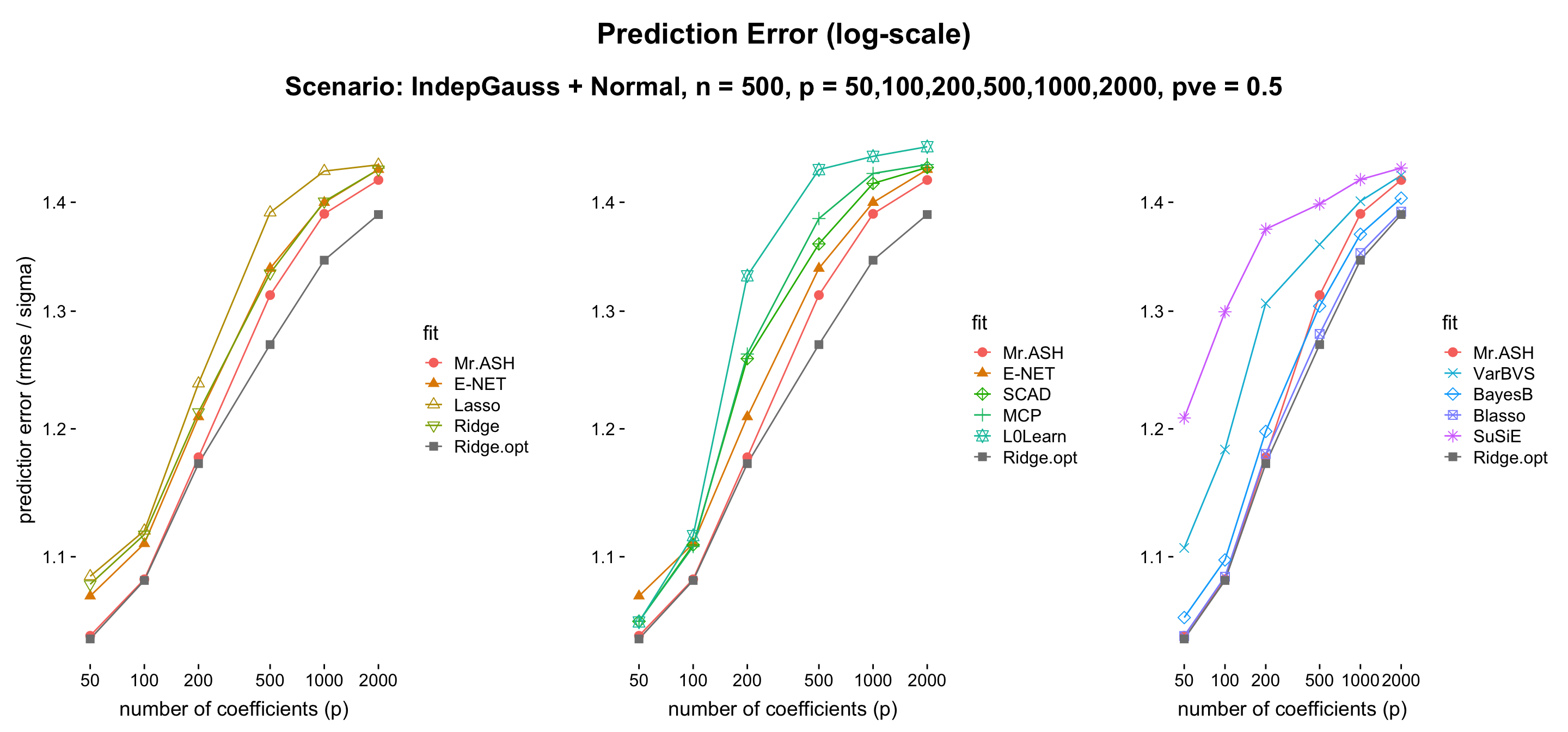
p4  = my.box2(sdat[sdat$fit != "Ridge.opt",], "fit", "time",
             gg_color_hue(13)[1:11]) +
  theme(axis.line    = element_blank(),
        axis.text.x  = element_text(angle = 45,hjust = 1),
        legend.position = "none") +
  scale_y_continuous(trans = "log10")
title     = ggdraw() + draw_label("Computation time (log-scale)", fontface = 'bold', size = 20)
subtitle  = ggdraw() + draw_label("Scenario: IndepGauss + Normal, n = 500, p = 50,100,200,500,1000,2000, pve = 0.5", fontface  = 'bold', size = 18) +
  labs(y = "computation time (sec)")
p0        = ggplot() + geom_blank() + theme_cowplot() + theme(axis.line = element_blank())
fig_main  = plot_grid(p0,p4,p0, nrow = 1, rel_widths = c(0.3,0.6,0.3))
fig       = plot_grid(title,subtitle,fig_main, ncol = 1, rel_heights = c(0.1,0.06,0.95))
fig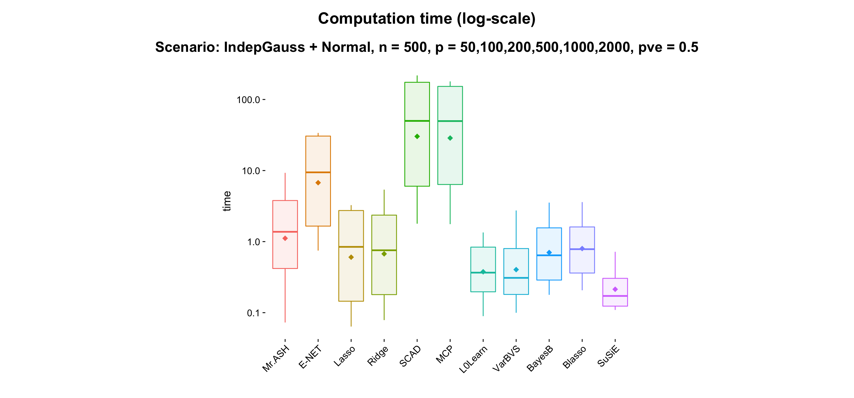
Source code
The source code will be popped up when you click code on the right side.
library(Matrix); library(ggplot2); library(cowplot); library(susieR); library(BGLR);
library(glmnet); library(mr.ash); library(ncvreg); library(L0Learn); library(varbvs);
standardize = FALSE
source('code/method_wrapper.R')
source('code/sim_wrapper.R')
tdat1        = list()
n            = 500
p_range      = c(50,100,200,500,1000,2000)
method_list  = c("varbvs","bayesb","blasso","susie","enet","lasso","ridge","scad","mcp","l0learn")
method_list2 = c("mr.ash", method_list, "ridge.opt")
method_num   = length(method_list) + 2
iter_num     = 20
pred         = matrix(0, iter_num, method_num);
time         = matrix(0, iter_num, method_num);
colnames(pred) <- colnames(time) <- method_list2

for (iter in 1:6) {
p               = p_range[iter]
for (i in 1:20) {
  data          = simulate_data(n, p, s = p, seed = i, signal = "normal", pve = 0.5)

  for (j in 1:length(method_list)) {
    fit.method    = get(paste("fit.",method_list[j],sep = ""))
    fit           = fit.method(data$X, data$y, data$X.test, data$y.test, seed = i)
    pred[i,j+1]   = fit$rsse / data$sigma / sqrt(n)
    time[i,j+1]   = fit$t

    if (method_list[j] == "lasso") {
      lasso.path.order = mr.ash:::path.order(fit$fit$glmnet.fit)
      lasso.beta       = as.vector(coef(fit$fit))[-1]
      lasso.time       = c(fit$t, fit$t2)
    }
  }

  fit         = fit.mr.ash(data$X, data$y, data$X.test, data$y.test, seed = i,
                           sa2 = (2^((0:19) / 5 / 2^iter) - 1)^2)
  pred[i,1]   = fit$rsse / data$sigma / sqrt(n)
  time[i,1]   = fit$t

  fit         = fit.ridge.opt(data$X, data$y, data$X.test, data$y.test, data$sigma, seed = i)
  pred[i,method_num] = fit$rsse / data$sigma / sqrt(n)
  time[i,method_num] = -Inf
  cat(i," ")
}
cat("\n")
print(c(colMeans(pred)))
tdat1[[iter]] = data.frame(pred = c(pred), time = c(time),
                           fit = rep(method_list2, each = 20))
}
System Configuration
Click the below Session Info.
sessionInfo()R version 3.5.3 (2019-03-11)
Platform: x86_64-apple-darwin15.6.0 (64-bit)
Running under: macOS High Sierra 10.13.3
Matrix products: default
BLAS: /Library/Frameworks/R.framework/Versions/3.5/Resources/lib/libRblas.0.dylib
LAPACK: /Library/Frameworks/R.framework/Versions/3.5/Resources/lib/libRlapack.dylib
locale:
[1] en_US.UTF-8/en_US.UTF-8/en_US.UTF-8/C/en_US.UTF-8/en_US.UTF-8
attached base packages:
[1] stats graphics grDevices utils datasets methods base
other attached packages:
[1] varbvs_2.6-5 L0Learn_1.1.0 ncvreg_3.11-1 mr.ash_0.1-2 glmnet_2.0-16
[6] foreach_1.4.4 BGLR_1.0.8 susieR_0.7.1 cowplot_0.9.4 ggplot2_3.2.1
[11] Matrix_1.2-17
loaded via a namespace (and not attached):
[1] Rcpp_1.0.2 RColorBrewer_1.1-2 plyr_1.8.4
[4] compiler_3.5.3 pillar_1.3.1 git2r_0.25.2
[7] workflowr_1.3.0 iterators_1.0.10 tools_3.5.3
[10] digest_0.6.18 evaluate_0.13 tibble_2.1.1
[13] gtable_0.3.0 lattice_0.20-38 pkgconfig_2.0.2
[16] rlang_0.4.0 yaml_2.2.0 xfun_0.6
[19] withr_2.1.2 stringr_1.4.0 dplyr_0.8.3
[22] knitr_1.22 fs_1.3.0 rprojroot_1.3-2
[25] grid_3.5.3 tidyselect_0.2.5 glue_1.3.1
[28] R6_2.4.0 rmarkdown_1.12 latticeExtra_0.6-28
[31] reshape2_1.4.3 purrr_0.3.2 magrittr_1.5
[34] whisker_0.3-2 codetools_0.2-16 backports_1.1.4
[37] scales_1.0.0 htmltools_0.4.0 assertthat_0.2.1
[40] colorspace_1.4-1 labeling_0.3 nor1mix_1.2-3
[43] stringi_1.4.3 lazyeval_0.2.2 munsell_0.5.0
[46] truncnorm_1.0-8 crayon_1.3.4