Result12_Initialization

Introduction

Design setting
Signal setting
PVE
Performance Measure
Packages / Libraries

Results

Source Code

Last updated: 2019-10-21

Checks: 7 0

Knit directory: mr-ash-workflow/

This reproducible R Markdown analysis was created with workflowr (version 1.4.0). The Checks tab describes the reproducibility checks that were applied when the results were created. The Past versions tab lists the development history.

R Markdown file: up-to-date

Great! Since the R Markdown file has been committed to the Git repository, you know the exact version of the code that produced these results.

Environment: empty

Great job! The global environment was empty. Objects defined in the global environment can affect the analysis in your R Markdown file in unknown ways. For reproduciblity it’s best to always run the code in an empty environment.

Seed: set.seed(20191007)

The command set.seed(20191007) was run prior to running the code in the R Markdown file. Setting a seed ensures that any results that rely on randomness, e.g. subsampling or permutations, are reproducible.

Session information: recorded

Great job! Recording the operating system, R version, and package versions is critical for reproducibility.

Cache: none

Nice! There were no cached chunks for this analysis, so you can be confident that you successfully produced the results during this run.

File paths: relative

Great job! Using relative paths to the files within your workflowr project makes it easier to run your code on other machines.

Repository version: 506cf21

Great! You are using Git for version control. Tracking code development and connecting the code version to the results is critical for reproducibility. The version displayed above was the version of the Git repository at the time these results were generated.

Note that you need to be careful to ensure that all relevant files for the analysis have been committed to Git prior to generating the results (you can use wflow_publish or wflow_git_commit). workflowr only checks the R Markdown file, but you know if there are other scripts or data files that it depends on. Below is the status of the Git repository when the results were generated:


Ignored files:
    Ignored:    .Rhistory
    Ignored:    .Rproj.user/
    Ignored:    analysis/ETA_1_lambda.dat
    Ignored:    analysis/ETA_1_parBayesB.dat
    Ignored:    analysis/mu.dat
    Ignored:    analysis/varE.dat

Untracked files:
    Untracked:  .DS_Store
    Untracked:  .Rapp.history
    Untracked:  docs/figure/Result9_Changepoint.Rmd/
    Untracked:  results/estsigma.RDS

Note that any generated files, e.g. HTML, png, CSS, etc., are not included in this status report because it is ok for generated content to have uncommitted changes.

These are the previous versions of the R Markdown and HTML files. If you’ve configured a remote Git repository (see ?wflow_git_remote), click on the hyperlinks in the table below to view them.

File	Version	Author	Date	Message
html	79e1aab	Youngseok	2019-10-17	Build site.
Rmd	2e3a7f5	Youngseok	2019-10-17	wflow_publish("analysis/*.Rmd")

Introduction

This .Rmd file is to plot results for the experiment MR.ASH and the comparison methods listed below.

glmnet R package: Ridge, Lasso, E-NET
ncvreg R package: SCAD, MCP
L0Learn R package: L0Learn
BGLR R package: BayesB, Blasso (Bayesian Lasso)
susieR R package: SuSiE (Sum of Single Effect)
varbvs R package: VarBVS (Variational Bayes Variable Selection)

The experiment is based on the following simulation setting.

Design setting

We use 20 real genotype matrices from GTEx consortium (https://gtexportal.org/home/).

$n = 287$ and $p = 5732, 7659, 6857, 4012, 6356, 8683, 4076, 7178, 4847, 5141, 6535, 7537, 7263, 7011, 7468, 5020, 8760, 5995, 6440, 5456$ . The number of coefficients $p$ varies from 4,012 to 8,760. The average size of $p$ is 6,401.3.

Also, columns of $X$ are very highly correlated (even some are perfectly correlated).

Signal setting

We sample the i.i.d. normal coefficients $\beta_j \sim N(0,\sigma_\beta^2)$ for $j \in J$ and $\beta_ j = 0$ otherwise, where $J$ is a set of randomly $s$ indices in $\{1,⋯,p\}$ c hosen uniformly at random.

This signal will be called sparsenormal.

We fix $s = 20$ throughout this experiment.

PVE

Then we sample $y = X\beta + \epsilon$ , where $\epsilon \sim N(0,\sigma^2 I_n)$ .

We fix PVE = 0.5, where PVE is the proportion of variance explained, defined by

${\rm PVE} = \frac{\textrm{Var}(X\beta)}{\textrm{Var}(X\beta) + \sigma^2},$ where $\textrm{Var}(a)$ denotes the sample variance of $a$ calculated using R function var. To this end, we set $\sigma^2 = \textrm{Var}(X\beta)$ .

Performance Measure

The above two figures display the prediction error. The prediction error we define here is

$\textrm{Pred.Err}(\hat\beta;y_{\rm test}, X_{\rm test}) = \frac{\textrm{RMSE}}{\sigma} = \frac{\|y_{\rm test} - X_{\rm test} \hat\beta \|}{\sqrt{n}\sigma}$ where $y_{\rm test}$ and $X_{\rm test}$ are test data sample in the same way. If $\hat\beta$ is fairly accurate, then we expect that $\rm RMSE$ is similar to $\sigma$ . Therefore in average $\textrm{Pred.Err} \geq 1$ and the smaller the better.

Packages / Libraries

A list of packages we have loaded is collapsed. Please click “code” to see the list.

library(Matrix); library(ggplot2); library(cowplot); library(susieR); library(BGLR);
library(glmnet); library(varbvs2); library(ncvreg); library(L0Learn); library(varbvs);
standardize = FALSE
source('code/method_wrapper.R')
source('code/sim_wrapper.R')

Results

sdat = readRDS("results/initialization1.RDS")
sdat$fit = factor(sdat$order, levels = c("null.init + increasing.order",
                                         "scad.init + increasing.order",
                                         "lasso.init + increasing.order",
                                         "lasso.init + lasso.pathorder",
                                         "lasso.init + scad.pathorder",
                                         "lasso.init + univar.absorder"))
                 
sdat$vobj = -sdat$vobj + sdat$vobj[1:20]

p1 = my.box(sdat, "fit", "vobj", values = col) +
  theme(axis.line    = element_blank(),
        axis.text.x  = element_text(angle = 45,hjust = 1),
        legend.position = "none")
subtitle  = ggdraw() + draw_label("Variational Objective", fontface  = 'bold', size = 18)
p1 = plot_grid(subtitle, p1, ncol = 1, rel_heights = c(0.06,0.95))

p2 = my.box(sdat, "fit", "pred", values = col) +
  theme(axis.line    = element_blank(),
        axis.text.x  = element_text(angle = 45,hjust = 1),
        legend.position = "none") +
  scale_y_continuous(trans = "log10", breaks = c(1,1.1,1.2,1.3)) +
  coord_cartesian(ylim = c(1,1.3))
subtitle  = ggdraw() + draw_label("Prediction Error", fontface  = 'bold', size = 18)
p2 = plot_grid(subtitle, p2, ncol = 1, rel_heights = c(0.06,0.95))

p3 = my.box(sdat, "fit", "time", values = col) +
  theme(axis.line    = element_blank(),
        axis.text.x  = element_text(angle = 45,hjust = 1),
        legend.position = "none") +
  scale_y_continuous(trans = "log10")
subtitle  = ggdraw() + draw_label("Computation Time", fontface  = 'bold', size = 18)
p3 = plot_grid(subtitle, p3, ncol = 1, rel_heights = c(0.06,0.95))

p4 = my.box(sdat, "fit", "numiter", values = col) +
  theme(axis.line    = element_blank(),
        axis.text.x  = element_text(angle = 45,hjust = 1),
        legend.position = "none") +
  scale_y_continuous(trans = "log10")
subtitle  = ggdraw() + draw_label("Number of Iterations", fontface  = 'bold', size = 18)
p4 = plot_grid(subtitle, p4, ncol = 1, rel_heights = c(0.06,0.95))
  
title     = ggdraw() + draw_label("Comparison of Update Orders (log-scale)", fontface = 'bold', size = 20) 
subtitle  = ggdraw() + draw_label("Scenario: EquiCorrGauss + SparseNormal, n = 500, p = 2000, s = 20, pve = 0.5, rho = 0.95", fontface  = 'bold', size = 18) 

fig_main  = plot_grid(p1,p2,p3,p4, nrow = 2, rel_widths = c(0.3,0.3,0.3))
fig       = plot_grid(title,subtitle,fig_main, ncol = 1, rel_heights = c(0.06,0.06,0.95))
fig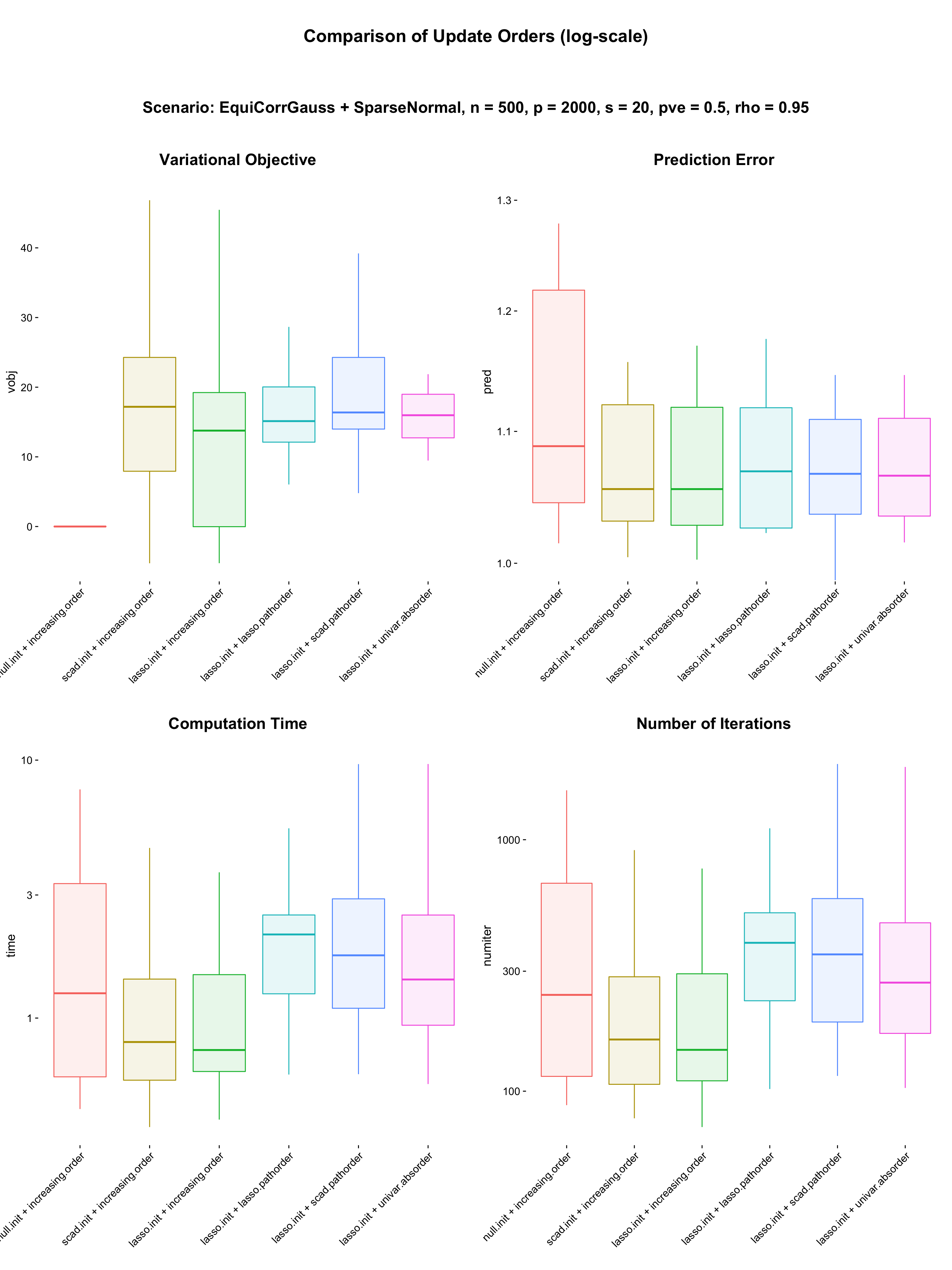

Version	Author	Date
79e1aab	Youngseok	2019-10-17

Source Code

tdat1        = list()
n            = 500
p            = 2000
s            = 20
sa2          = (2^((0:19) / 20) - 1)^2
method_list  = c("null.init + increasing.order","lasso.init + increasing.order",
                 "scad.init + increasing.order",
                 "lasso.init + lasso.pathorder", "lasso.init + scad.pathorder",
                 "lasso.init + univar.absorder")
method_num   = length(method_list)
iter_num     = 20
pred         = matrix(0, iter_num, method_num); colnames(pred) = method_list
time         = matrix(0, iter_num, method_num); colnames(time) = method_list
numiter      = matrix(0, iter_num, method_num); colnames(numiter) = method_list
vobj         = matrix(0, iter_num, method_num); colnames(vobj) = method_list


for (i in 1:iter_num) {
  data          = simulate_data(n, p, s = s, seed = i, signal = "normal", rho = 0.95,
                                design = "equicorrgauss", pve = 0.5)
  X             = data$X
  y             = data$y

  fit.lasso        <- cv.glmnet(x = X, y = y, standardize = standardize)
  fit.lasso$beta    = coef(fit.lasso)[-1]
      
  t.blasso          = system.time(
  fit.blasso       <- BGLR(y, ETA = list(list(X = X, model="BL", standardize = standardize)),
                           verbose = FALSE))
  fit.blasso$beta   = c(fit.blasso$ETA[[1]]$b)
  
  

  t.mrash1          = system.time(
  fit.mrash1       <- mr_ash(X = X, y = y, sa2 = sa2,
                             stepsize = 1, max.iter = 2000,
                             standardize = standardize, beta.init = NULL,
                             tol = list(epstol = 1e-12, convtol = 1e-8)))
  t.mrash2          = system.time(
  fit.mrash2       <- mr_ash(X = X, y = y, sa2 = sa2,
                             stepsize = 1, max.iter = 2000,
                             standardize = standardize, beta.init = fit.lasso$beta,
                             tol = list(epstol = 1e-12, convtol = 1e-8)))
  t.mrash3          = system.time(
  fit.mrash3       <- mr_ash(X = X, y = y, sa2 = sa2,
                             stepsize = 1, max.iter = 2000,
                             standardize = standardize, beta.init = fit.scad$beta,
                             tol = list(epstol = 1e-12, convtol = 1e-8)))
  t.mrash4          = system.time(
  fit.mrash4       <- mr_ash_order(X = X, y = y, sa2 = sa2,
                                   stepsize = 1, max.iter = 2000,
                                   standardize = standardize, beta.init = fit.lasso$beta,
                                   order = "manual",
                                   o = rep(lasso.pathorder, 2000),
                                   tol = list(epstol = 1e-12, convtol = 1e-8)))
  t.mrash5          = system.time(
  fit.mrash5       <- mr_ash_order(X = X, y = y, sa2 = sa2,
                                   stepsize = 1, max.iter = 2000,
                                   standardize = standardize, beta.init = fit.lasso$beta,
                                   order = "manual",
                                   o = rep(scad.pathorder, 2000),
                                   tol = list(epstol = 1e-12, convtol = 1e-8)))
  t.mrash6          = system.time(
  fit.mrash6       <- mr_ash_order(X = X, y = y, sa2 = sa2,
                                   stepsize = 1, max.iter = 2000,
                                   standardize = standardize, beta.init = fit.lasso$beta,
                                   order = "manual",
                                   o = rep(univar.absorder, 2000),
                                   tol = list(epstol = 1e-12, convtol = 1e-8)))
 
  for (j in 1:6) {
    fit           = get(paste("fit.mrash",j,sep = ""))
    pred[i,j]     = norm(data$y.test - predict(fit, data$X.test), '2') / sqrt(500) / data$sigma
    numiter[i,j]  = fit$iter
    vobj[i,j]     = fit$varobj[fit$iter]
    time[i,j]     = get(paste("t.mrash",j,sep = ""))[3]
  }
  
  print(c(pred[i,]))
}

tdat1 = data.frame(pred = c(pred), vobj = c(vobj), time = c(time),
                   numiter = c(numiter),
                   order = rep(method_list, each = 20))

sessionInfo()

R version 3.5.3 (2019-03-11)
Platform: x86_64-apple-darwin15.6.0 (64-bit)
Running under: macOS Mojave 10.14

Matrix products: default
BLAS: /Library/Frameworks/R.framework/Versions/3.5/Resources/lib/libRblas.0.dylib
LAPACK: /Library/Frameworks/R.framework/Versions/3.5/Resources/lib/libRlapack.dylib

locale:
[1] en_US.UTF-8/en_US.UTF-8/en_US.UTF-8/C/en_US.UTF-8/en_US.UTF-8

attached base packages:
[1] stats     graphics  grDevices utils     datasets  methods   base     

other attached packages:
 [1] varbvs_2.5-16 L0Learn_1.2.0 ncvreg_3.11-1 varbvs2_0.1-1 glmnet_2.0-18
 [6] foreach_1.4.7 BGLR_1.0.8    susieR_0.8.0  cowplot_1.0.0 ggplot2_3.2.1
[11] Matrix_1.2-17

loaded via a namespace (and not attached):
 [1] Rcpp_1.0.2          RColorBrewer_1.1-2  plyr_1.8.4         
 [4] compiler_3.5.3      pillar_1.4.2        git2r_0.26.1       
 [7] workflowr_1.4.0     iterators_1.0.12    tools_3.5.3        
[10] digest_0.6.21       evaluate_0.14       tibble_2.1.3       
[13] gtable_0.3.0        lattice_0.20-38     pkgconfig_2.0.3    
[16] rlang_0.4.0         yaml_2.2.0          xfun_0.9           
[19] withr_2.1.2         stringr_1.4.0       dplyr_0.8.3        
[22] knitr_1.25          fs_1.3.1            rprojroot_1.3-2    
[25] grid_3.5.3          tidyselect_0.2.5    glue_1.3.1         
[28] R6_2.4.0            rmarkdown_1.15      latticeExtra_0.6-28
[31] reshape2_1.4.3      purrr_0.3.2         magrittr_1.5       
[34] whisker_0.4         codetools_0.2-16    backports_1.1.4    
[37] scales_1.0.0        htmltools_0.3.6     assertthat_0.2.1   
[40] colorspace_1.4-1    labeling_0.3        nor1mix_1.3-0      
[43] stringi_1.4.3       lazyeval_0.2.2      munsell_0.5.0      
[46] truncnorm_1.0-8     crayon_1.3.4