Example 2: RSS-BVSR with Various LD Matrices
Xiang Zhu
Last updated: 2020-06-24
Checks: 2 0
Knit directory: rss/
This reproducible R Markdown analysis was created with workflowr (version 1.6.2). The Checks tab describes the reproducibility checks that were applied when the results were created. The Past versions tab lists the development history.
Great! Since the R Markdown file has been committed to the Git repository, you know the exact version of the code that produced these results.
Great! You are using Git for version control. Tracking code development and connecting the code version to the results is critical for reproducibility.
The results in this page were generated with repository version 1e806af. See the Past versions tab to see a history of the changes made to the R Markdown and HTML files.
Note that you need to be careful to ensure that all relevant files for the analysis have been committed to Git prior to generating the results (you can use wflow_publish or wflow_git_commit). workflowr only checks the R Markdown file, but you know if there are other scripts or data files that it depends on. Below is the status of the Git repository when the results were generated:
Ignored files:
    Ignored:    .Rproj.user/
    Ignored:    .spelling
    Ignored:    examples/example5/.Rhistory
    Ignored:    examples/example5/Aseg_chr16.mat
    Ignored:    examples/example5/example5_simulated_data.mat
    Ignored:    examples/example5/example5_simulated_results.mat
    Ignored:    examples/example5/ibd2015_path2641_genes_results.mat

Untracked files:
    Untracked:  docs_old/

Unstaged changes:
    Modified:   rmd/_site.yml
Note that any generated files, e.g. HTML, png, CSS, etc., are not included in this status report because it is ok for generated content to have uncommitted changes.
These are the previous versions of the repository in which changes were made to the R Markdown (rmd/example_2.Rmd) and HTML (docs/example_2.html) files. If you’ve configured a remote Git repository (see ?wflow_git_remote), click on the hyperlinks in the table below to view the files as they were in that past version.
| File | Version | Author | Date | Message |
|---|---|---|---|---|
| html | 9c00612 | Xiang Zhu | 2020-06-23 | Build site. |
| Rmd | e4bd120 | Xiang Zhu | 2020-06-23 | wflow_publish(“rmd/example_2.Rmd”) |
| html | 91c0f75 | Xiang Zhu | 2020-06-23 | Build site. |
| Rmd | 8fed651 | Xiang Zhu | 2020-06-23 | wflow_publish(“rmd/example_2.Rmd”) |
Overview
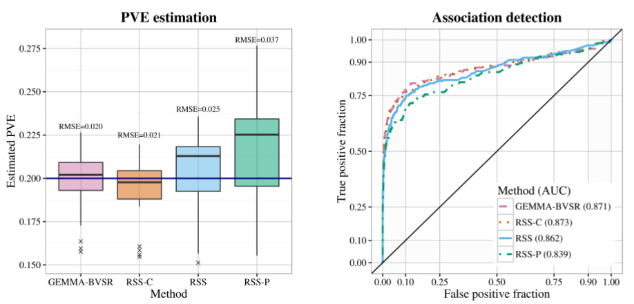
This example illustrates the impact of different LD estimates on the RSS results. Three types of estimated LD matrices are considered: cohort sample LD, panel sample LD and shrinkage panel sample LD in Wen and Stephens, (2010) This example is closely related to Section 4.1 of Zhu and Stephens (2017).
The single-SNP summary-level data are computed from a simulated GWAS dataset. The simulation scheme is described in Section 4.1 Zhu and Stephens (2017). Specifically, 10 “causal” SNPs are randomly drawn from 982 SNPs on chromosome 16, with effect sizes coming from standard normal \({\cal N}(0,1)\). Effect sizes of remaining SNPs are zero. The true PVE (SNP heritability) is 0.2.
Three types of LD estimates are considered here.
cohort sample LD: the sample correlation matrix using genotypes in the cohort (WTCCC UK Blood Service Control Group)
shrinkage panel sample LD: the shrinkage correlation matrix (Wen and Stephens, 2010) using genotypes in the panel (WTCCC 1958 British Birth Cohort)
panel sample LD: the sample correlation matrix using genotypes in the panel (WTCCC 1958 British Birth Cohort)
To reproduce results of Example 2, please read the step-by-step guide below and run example2.m. Before running example2.m, please first install the MCMC subroutines. Please find installation instructions here.
Step-by-step illustration
Step 1. Download the simulated single-SNP summary-level data and LD estimates example2.mat. Please contact me if you have trouble accessing these files.
The data file example2.mat contains the following elements.
betahat: 982 by 1 vector, single-SNP effect size estimate for each SNPse: 982 by 1 vector, standard errors of the single-SNP effect size estimatesNsnp: 982 by 1 vector, sample size of each SNPcohort_R: cohort sample LDshrink_R: shrinkage panel sample LDpanel_R: panel sample LDsnp_info: 3 by 1 cell, ID and allele of each SNP
Step 2. Fit three RSS-BVSR models with different LD matrices.
% cohort sample LD
[betasam, gammasam, hsam, logpisam, Naccept] = rss_bvsr(betahat, se, cohort_R, Nsnp, Ndraw, Nburn, Nthin);

% shrinkage panel sample LD
[betasam, gammasam, hsam, logpisam, Naccept] = rss_bvsr(betahat, se, shrink_R, Nsnp, Ndraw, Nburn, Nthin);

% panel sample LD
[betasam, gammasam, hsam, logpisam, Naccept] = rss_bvsr(betahat, se, panel_R, Nsnp, Ndraw, Nburn, Nthin);
More simulations
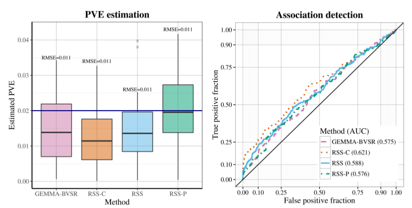
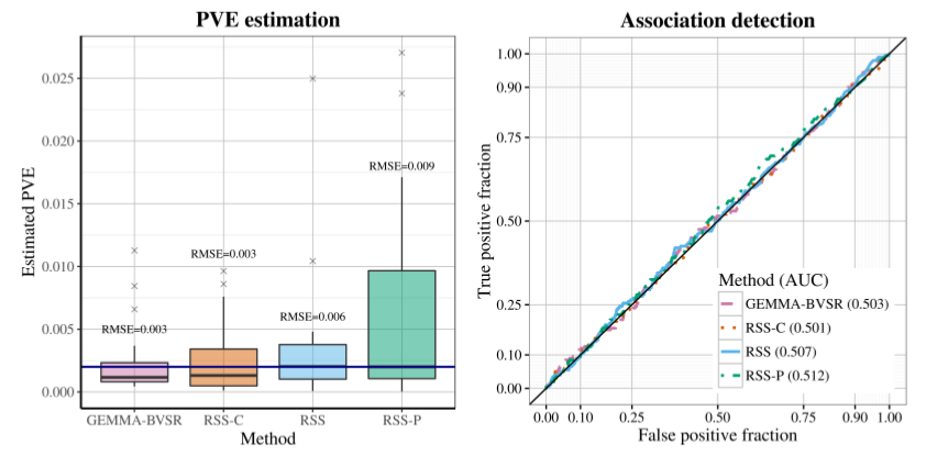
The simulations in Section 4.1 of Zhu and Stephens (2017) are essentially “replications” of the example above. To facilitate reproducible research, we make the simulated datasets in Section 4.1 available1.
Each simulated dataset contains three files: genotype.txt, phenotype.txt and simulated_data.mat. The files genotype.txt and phenotype.txt are the genotype and phenotype files for GEMMA. The file simulated_data.mat contains three cells.
true_para = {pve, beta, gamma, sigma};
individual_data = {y, X};
summary_data = {betahat, se, Nsnp};
Only the summary_data cell above is used as the input for RSS methods.
RSS methods also require an estimated LD matrix. The three types of LD matrices are provided in the file genotype2.mat1.
After applying RSS methods to these simulated data, we obtain the following results.
| True PVE = 0.2 |
|---|
 |
| True PVE = 0.02 | True PVE = 0.002 |
|---|---|
 |
 |
Footnotes:
- Currently these files are locked, since they contain individual-level genotypes from Wellcome Trust Case Control Consortium (WTCCC, https://www.wtccc.org.uk/). You need to get permission from WTCCC before we can share these files with you.