Clustering Cusanovich et al (2018) data using topic proportions with K = 13
Kaixuan Luo
Last updated: 2020-10-21
Checks: 6 1
Knit directory: scATACseq-topics/
This reproducible R Markdown analysis was created with workflowr (version 1.6.2). The Checks tab describes the reproducibility checks that were applied when the results were created. The Past versions tab lists the development history.
Great! Since the R Markdown file has been committed to the Git repository, you know the exact version of the code that produced these results.
Great job! The global environment was empty. Objects defined in the global environment can affect the analysis in your R Markdown file in unknown ways. For reproduciblity it’s best to always run the code in an empty environment.
The command set.seed(20200729) was run prior to running the code in the R Markdown file. Setting a seed ensures that any results that rely on randomness, e.g. subsampling or permutations, are reproducible.
Great job! Recording the operating system, R version, and package versions is critical for reproducibility.
- kmeans-1
- kmeans-2
- kmeans-3
To ensure reproducibility of the results, delete the cache directory clusters_Cusanovich2018_k13_cache and re-run the analysis. To have workflowr automatically delete the cache directory prior to building the file, set delete_cache = TRUE when running wflow_build() or wflow_publish().
Great job! Using relative paths to the files within your workflowr project makes it easier to run your code on other machines.
Great! You are using Git for version control. Tracking code development and connecting the code version to the results is critical for reproducibility.
The results in this page were generated with repository version 82292d5. See the Past versions tab to see a history of the changes made to the R Markdown and HTML files.
Note that you need to be careful to ensure that all relevant files for the analysis have been committed to Git prior to generating the results (you can use wflow_publish or wflow_git_commit). workflowr only checks the R Markdown file, but you know if there are other scripts or data files that it depends on. Below is the status of the Git repository when the results were generated:
Ignored files:
    Ignored:    .Rhistory
    Ignored:    .Rproj.user/
    Ignored:    analysis/clusters_Cusanovich2018_k13_cache/
    Ignored:    analysis/figure/

Untracked files:
    Untracked:  analysis/clusters_pca_structure_Cusanovich2018.Rmd

Unstaged changes:
    Modified:   analysis/assess_fits_Lareau2019_bonemarrow.Rmd
    Modified:   code/plots.R
    Modified:   scripts/fit_all_models_Lareau2019.sh
Note that any generated files, e.g. HTML, png, CSS, etc., are not included in this status report because it is ok for generated content to have uncommitted changes.
These are the previous versions of the repository in which changes were made to the R Markdown (analysis/clusters_Cusanovich2018_k13.Rmd) and HTML (docs/clusters_Cusanovich2018_k13.html) files. If you’ve configured a remote Git repository (see ?wflow_git_remote), click on the hyperlinks in the table below to view the files as they were in that past version.
| File | Version | Author | Date | Message |
|---|---|---|---|---|
| Rmd | 82292d5 | kevinlkx | 2020-10-21 | update colors and interpret clusters with tissue labels |
| html | b8a48b9 | kevinlkx | 2020-10-20 | Build site. |
| Rmd | a4daf6d | kevinlkx | 2020-10-20 | clustering with k = 13 topics |
| html | ac8ca65 | kevinlkx | 2020-10-20 | Build site. |
| Rmd | 98920ed | kevinlkx | 2020-10-20 | clustering with k = 13 topics |
| html | a38788b | kevinlkx | 2020-10-20 | Build site. |
| Rmd | f8bea96 | kevinlkx | 2020-10-20 | clustering with k = 13 topics |
Here we explore the structure in the Cusanovich et al (2018) ATAC-seq data inferred from the multinomial topic model with \(k = 13\).
Load packages and some functions used in this analysis.
library(Matrix)
library(dplyr)
library(ggplot2)
library(cowplot)
library(fastTopics)
source("code/plots.R")
Load the data. The counts are no longer needed at this stage of the analysis.
data.dir <- "/project2/mstephens/kevinluo/scATACseq-topics/data/Cusanovich_2018/processed_data/"
load(file.path(data.dir, "Cusanovich_2018.RData"))
rm(counts)
Plot PCs of the topic proportions
We first use PCA to explore the structure inferred from the multinomial topic model with \(k = 13\):
Load the \(k = 13\) Poisson NMF fit.
out.dir <- "/project2/mstephens/kevinluo/scATACseq-topics/output/Cusanovich_2018"
fit <- readRDS(file.path(out.dir, "/fit-Cusanovich2018-scd-ex-k=13.rds"))$fit
Plot PCs of the topic proportions.
p.pca1.1 <- pca_plot(poisson2multinom(fit),pcs = 1:2,fill = "none")
p.pca1.2 <- pca_plot(poisson2multinom(fit),pcs = 3:4,fill = "none")
p.pca1.3 <- pca_plot(poisson2multinom(fit),pcs = 5:6,fill = "none")
p.pca1.4 <- pca_plot(poisson2multinom(fit),pcs = 7:8,fill = "none")
p.pca1.5 <- pca_plot(poisson2multinom(fit),pcs = 9:10,fill = "none")
p.pca1.6 <- pca_plot(poisson2multinom(fit),pcs = 11:12,fill = "none")

plot_grid(p.pca1.1,p.pca1.2,p.pca1.3,p.pca1.4,p.pca1.5,p.pca1.6)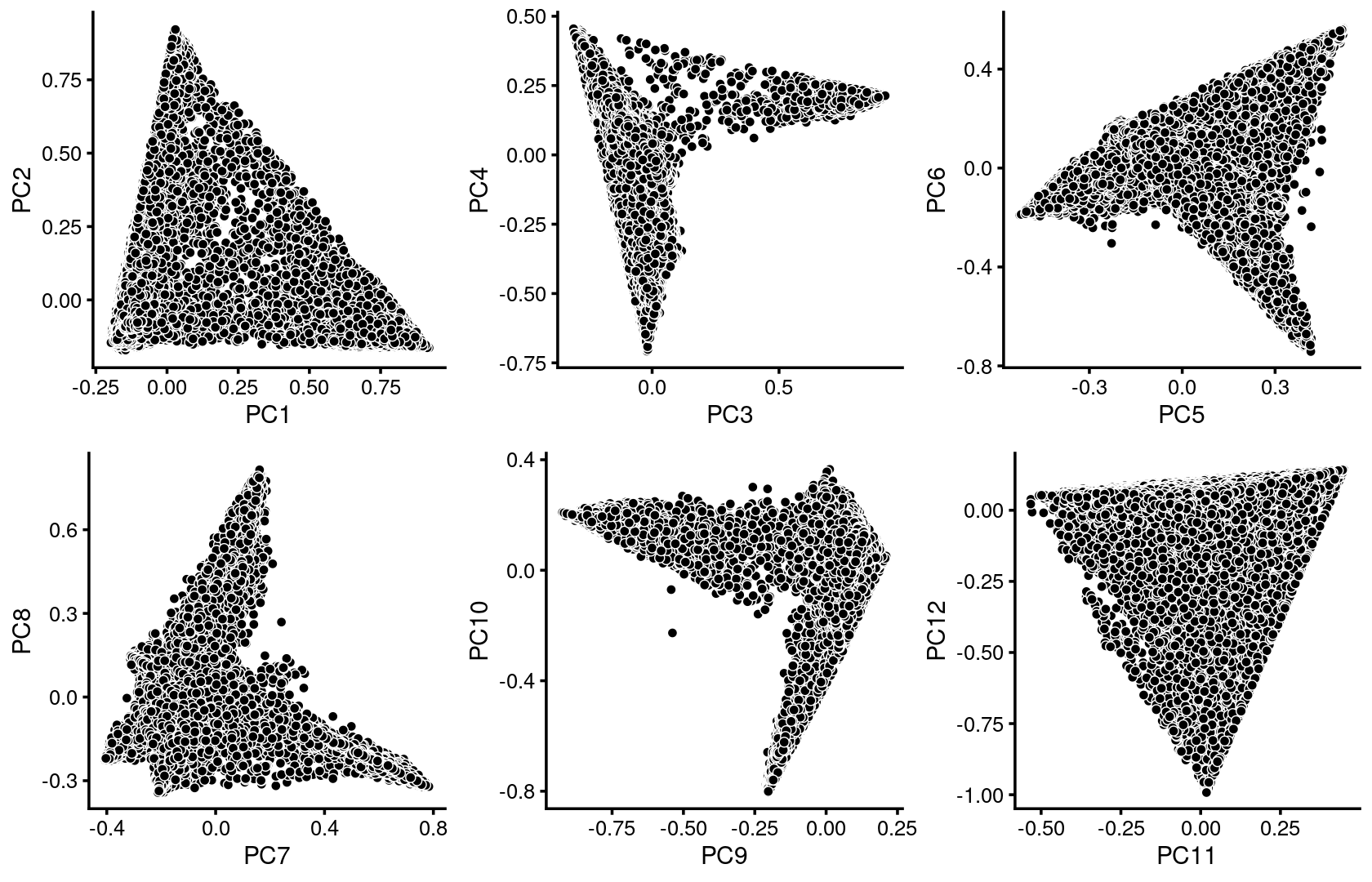
| Version | Author | Date |
|---|---|---|
| a38788b | kevinlkx | 2020-10-20 |
Some of the structure is more evident from “hexbin” plots showing the density of the points.
breaks <- c(0,1,5,10,100,Inf)
p.pca2.1 <- pca_hexbin_plot(poisson2multinom(fit), pcs = 1:2, breaks = breaks) + guides(fill = "none")
p.pca2.2 <- pca_hexbin_plot(poisson2multinom(fit), pcs = 3:4, breaks = breaks) + guides(fill = "none")
p.pca2.3 <- pca_hexbin_plot(poisson2multinom(fit), pcs = 5:6, breaks = breaks) + guides(fill = "none")
p.pca2.4 <- pca_hexbin_plot(poisson2multinom(fit), pcs = 7:8, breaks = breaks) + guides(fill = "none")
p.pca2.5 <- pca_hexbin_plot(poisson2multinom(fit), pcs = 9:10, breaks = breaks) + guides(fill = "none")
p.pca2.6 <- pca_hexbin_plot(poisson2multinom(fit), pcs = 11:12, breaks = breaks) + guides(fill = "none")

plot_grid(p.pca2.1,p.pca2.2,p.pca2.3,p.pca2.4,p.pca2.5,p.pca2.6)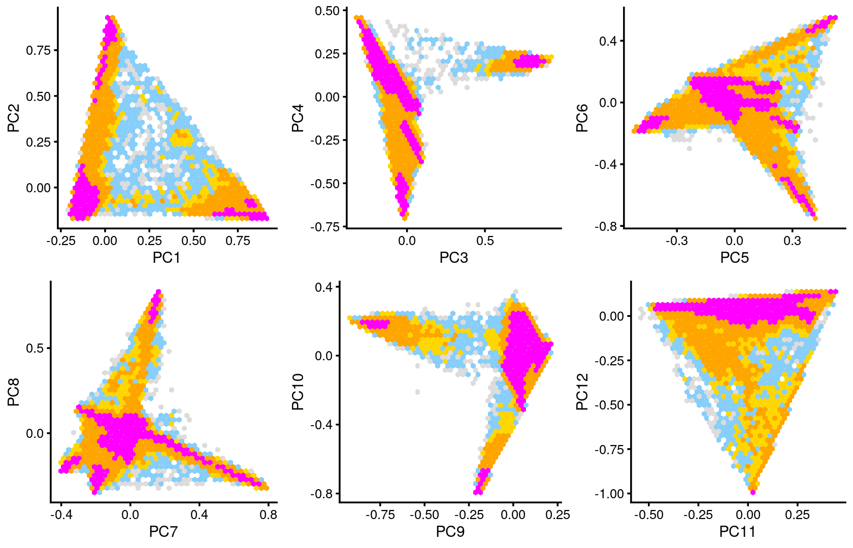
| Version | Author | Date |
|---|---|---|
| a38788b | kevinlkx | 2020-10-20 |
Layer the tissue and cell labels onto the PC plots
Next, we layer the tissue and cell labels onto the PC plots.
PCs 1 and 2:
p.pca3.1 <- labeled_pca_plot(fit,1:2,samples$tissue,font_size = 7,
                       legend_label = "tissue")
p.pca3.2 <- labeled_pca_plot(fit,1:2,samples$cell_label,font_size = 7,
                        legend_label = "cell_label")
plot_grid(p.pca3.1,p.pca3.2,rel_widths = c(8,11))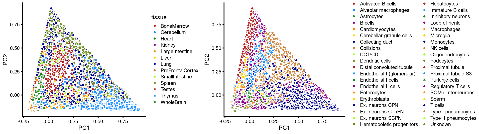
| Version | Author | Date |
|---|---|---|
| a38788b | kevinlkx | 2020-10-20 |
PCs 3 and 4:
p.pca3.3 <- labeled_pca_plot(fit,3:4,samples$tissue,font_size = 7,
                        legend_label = "tissue")
p.pca3.4 <- labeled_pca_plot(fit,3:4,samples$cell_label,font_size = 7,
                        legend_label = "cell_label")
plot_grid(p.pca3.3,p.pca3.4,rel_widths = c(8,11))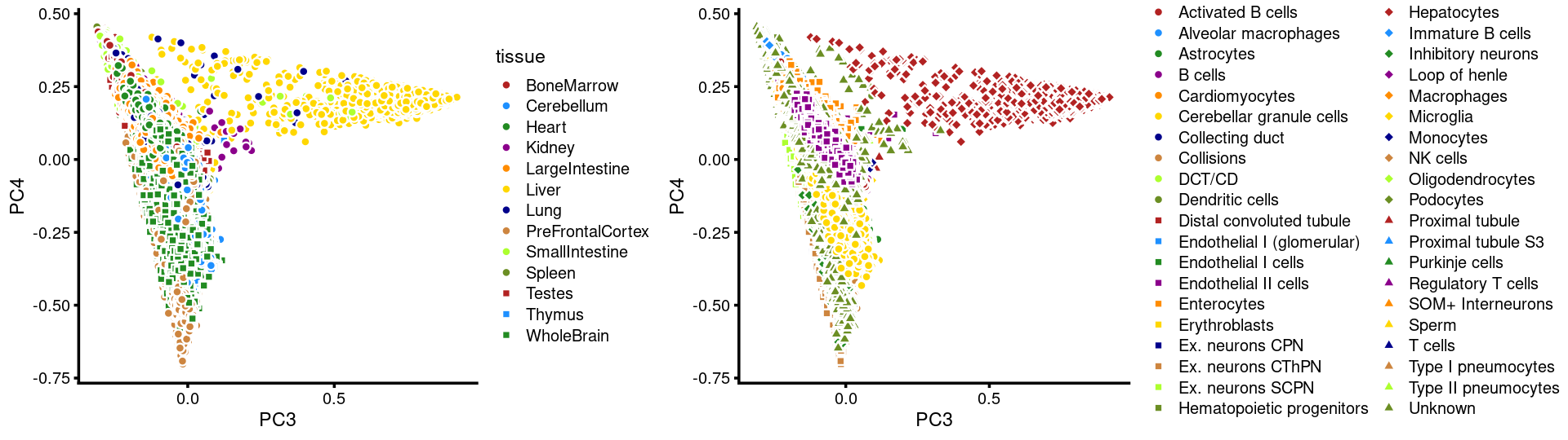
| Version | Author | Date |
|---|---|---|
| a38788b | kevinlkx | 2020-10-20 |
PCs 5 and 6:
p.pca3.5 <- labeled_pca_plot(fit,5:6,samples$tissue,font_size = 7,
                       legend_label = "tissue")
p.pca3.6 <- labeled_pca_plot(fit,5:6,samples$cell_label,font_size = 7,
                        legend_label = "cell_label")
plot_grid(p.pca3.5,p.pca3.6,rel_widths = c(8,11))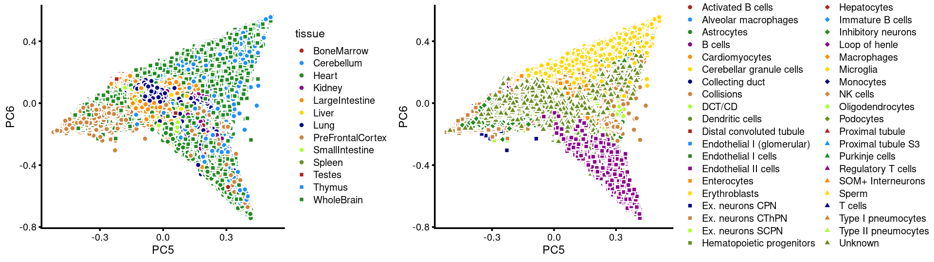
| Version | Author | Date |
|---|---|---|
| a38788b | kevinlkx | 2020-10-20 |
PCs 7 and 8:
p.pca3.7 <- labeled_pca_plot(fit,7:8,samples$tissue,font_size = 7,
                       legend_label = "tissue")
p.pca3.8 <- labeled_pca_plot(fit,7:8,samples$cell_label,font_size = 7,
                        legend_label = "cell_label")
plot_grid(p.pca3.7,p.pca3.8,rel_widths = c(8,11))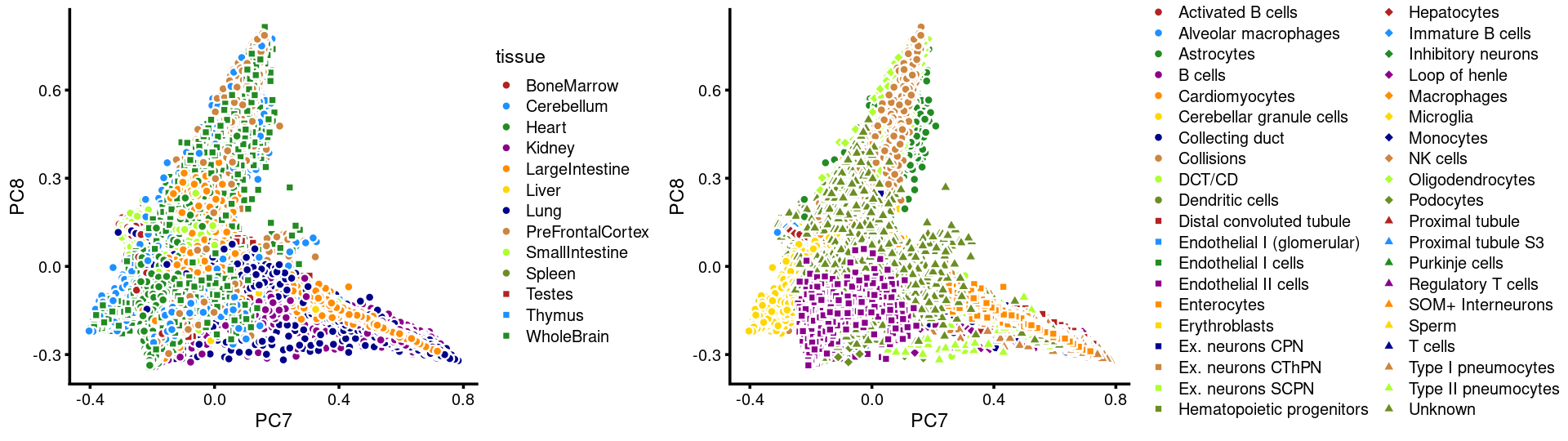
| Version | Author | Date |
|---|---|---|
| a38788b | kevinlkx | 2020-10-20 |
PCs 9 and 10:
p.pca3.9 <- labeled_pca_plot(fit,9:10,samples$tissue,font_size = 7,
                       legend_label = "tissue")
p.pca3.10 <- labeled_pca_plot(fit,9:10,samples$cell_label,font_size = 7,
                        legend_label = "cell_label")
plot_grid(p.pca3.9,p.pca3.10,rel_widths = c(8,11))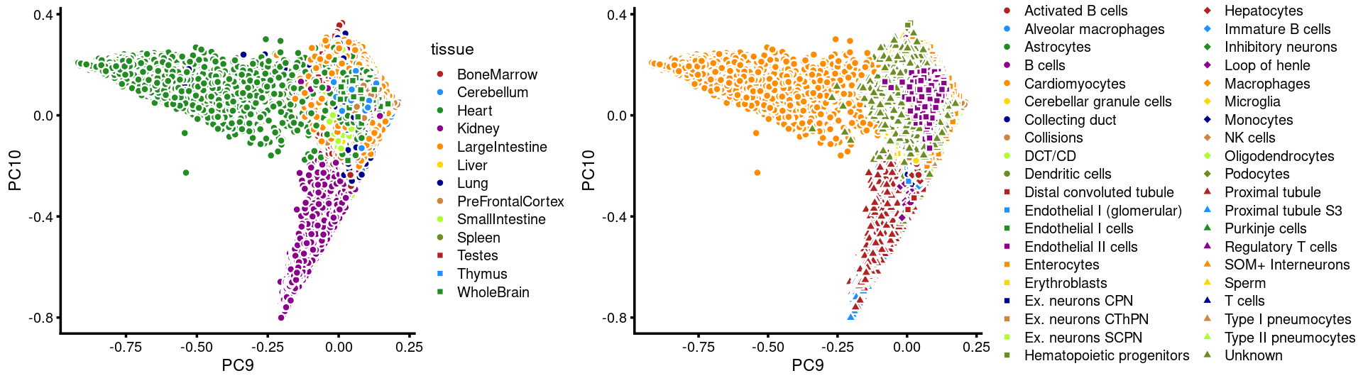
| Version | Author | Date |
|---|---|---|
| a38788b | kevinlkx | 2020-10-20 |
PCs 11 and 12:
p.pca3.11 <- labeled_pca_plot(fit,11:12,samples$tissue,font_size = 7,
                       legend_label = "tissue")
p.pca3.12 <- labeled_pca_plot(fit,11:12,samples$cell_label,font_size = 7,
                        legend_label = "cell_label")
plot_grid(p.pca3.11,p.pca3.12,rel_widths = c(8,11))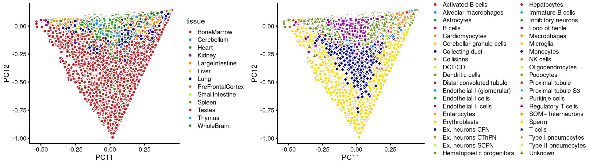
| Version | Author | Date |
|---|---|---|
| a38788b | kevinlkx | 2020-10-20 |
Visualize by structure plot grouped by tissues
set.seed(10)
colors_topics <- c("#a6cee3","#1f78b4","#b2df8a","#33a02c","#fb9a99","#e31a1c",
                   "#fdbf6f","#ff7f00","#cab2d6","#6a3d9a","#ffff99","#b15928",
                   "gray")
rows <- sample(nrow(fit$L),4000)
samples$tissue <- as.factor(samples$tissue)

p.structure.1 <- structure_plot(select(poisson2multinom(fit),loadings = rows),
                     grouping = samples[rows, "tissue"],n = Inf,gap = 20,
                     perplexity = 50,topics = 1:13,colors = colors_topics,
                     num_threads = 4,verbose = FALSE)
# Perplexity automatically changed to 35 because original setting of 50 was too large for the number of samples (111)
# Perplexity automatically changed to 41 because original setting of 50 was too large for the number of samples (128)

print(p.structure.1)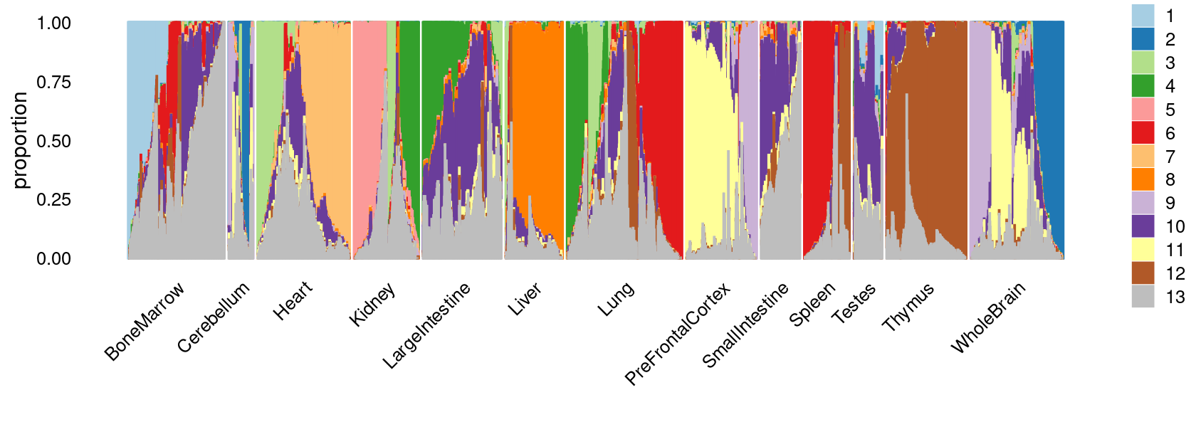
k-means clustering on topic proportions
Define clusters using k-means, and then create structure plot based on the clusters from k-means.
Define clusters using k-means with \(k = 14\):
set.seed(10)

clusters.14 <- factor(kmeans(poisson2multinom(fit)$L,centers = 14)$cluster)
print(sort(table(clusters.14),decreasing = TRUE))
# clusters.14
#    13     7     3     2     4     1    12    10     8    14     5     6    11
# 18096 10936  9331  7693  6077  5817  4184  3994  3627  3306  2964  2821  2073
#     9
#   254
Warning: The above code chunk cached its results, but it won’t be re-run if previous chunks it depends on are updated. If you need to use caching, it is highly recommended to also set knitr::opts_chunk$set(autodep = TRUE) at the top of the file (in a chunk that is not cached). Alternatively, you can customize the option dependson for each individual chunk that is cached. Using either autodep or dependson will remove this warning. See the knitr cache options for more details.
Structure plot based on k-means clusters
colors_topics <- c("#a6cee3","#1f78b4","#b2df8a","#33a02c","#fb9a99","#e31a1c",
                   "#fdbf6f","#ff7f00","#cab2d6","#6a3d9a","#ffff99","#b15928",
                   "gray")
rows <- sample(nrow(fit$L),4000)

p.structure.2 <- structure_plot(select(poisson2multinom(fit),loadings = rows),
                     grouping = clusters.14[rows],n = Inf,gap = 20,
                     perplexity = 50,topics = 1:13,colors = colors_topics,
                     num_threads = 4,verbose = FALSE)
# Perplexity automatically changed to 42 because original setting of 50 was too large for the number of samples (131)
# Perplexity automatically changed to 1 because original setting of 50 was too large for the number of samples (7)
# Perplexity automatically changed to 26 because original setting of 50 was too large for the number of samples (82)
# Perplexity automatically changed to 44 because original setting of 50 was too large for the number of samples (137)
print(p.structure.2)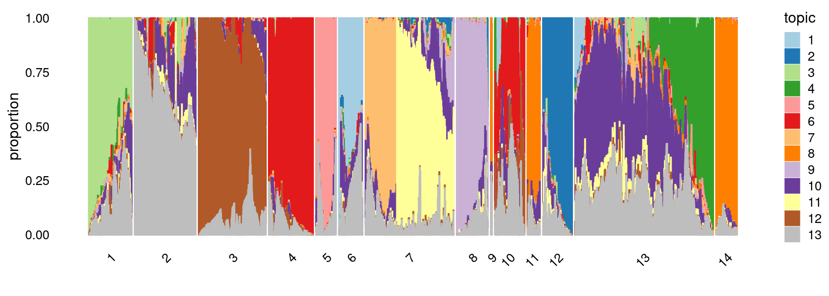
| Version | Author | Date |
|---|---|---|
| a38788b | kevinlkx | 2020-10-20 |
Define clusters using k-means with \(k = 15\):
set.seed(10)

clusters.15 <- factor(kmeans(poisson2multinom(fit)$L,centers = 15)$cluster)
print(sort(table(clusters.15),decreasing = TRUE))
# clusters.15
#    13     7     3     9     8     4     1    14    12     2    15     5     6
# 14936  8426  8043  6796  6757  5951  5784  4314  4168  3657  3649  2960  2738
#    10    11
#  1697  1297
Warning: The above code chunk cached its results, but it won’t be re-run if previous chunks it depends on are updated. If you need to use caching, it is highly recommended to also set knitr::opts_chunk$set(autodep = TRUE) at the top of the file (in a chunk that is not cached). Alternatively, you can customize the option dependson for each individual chunk that is cached. Using either autodep or dependson will remove this warning. See the knitr cache options for more details.
Structure plot based on k-means clusters
colors_topics <- c("#a6cee3","#1f78b4","#b2df8a","#33a02c","#fb9a99","#e31a1c",
            "#fdbf6f","#ff7f00","#cab2d6","#6a3d9a","#ffff99","#b15928",
            "gray")
rows <- sample(nrow(fit$L),4000)

p.structure.3 <- structure_plot(select(poisson2multinom(fit),loadings = rows),
                     grouping = clusters.15[rows],n = Inf,gap = 20,
                     perplexity = 50,topics = 1:13,colors = colors_topics,
                     num_threads = 4,verbose = FALSE)
# Perplexity automatically changed to 42 because original setting of 50 was too large for the number of samples (131)
# Perplexity automatically changed to 48 because original setting of 50 was too large for the number of samples (149)
# Perplexity automatically changed to 23 because original setting of 50 was too large for the number of samples (75)
# Perplexity automatically changed to 13 because original setting of 50 was too large for the number of samples (44)
print(p.structure.3)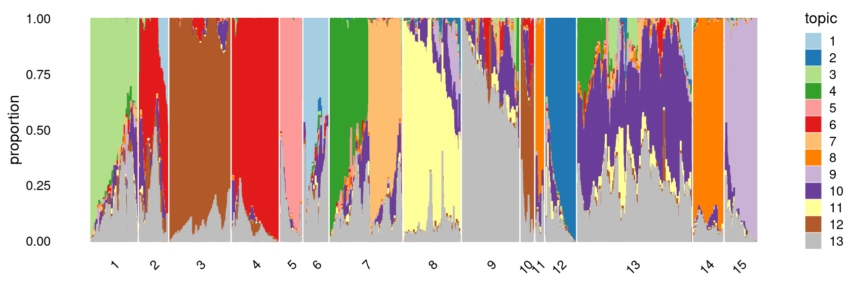
| Version | Author | Date |
|---|---|---|
| a38788b | kevinlkx | 2020-10-20 |
Define clusters using k-means with \(k = 20\):
set.seed(10)

clusters.20 <- factor(kmeans(poisson2multinom(fit)$L,centers = 20)$cluster)
print(sort(table(clusters.20),decreasing = TRUE))
# clusters.20
#    17    13     4     1     3    20     8    12     7     2    15    14    18
# 13635  6703  5963  5809  5557  5057  5045  4012  3783  3492  3490  3147  2989
#     5     6    11    16    10    19     9
#  2958  2738  2158  1839  1756   721   321
Warning: The above code chunk cached its results, but it won’t be re-run if previous chunks it depends on are updated. If you need to use caching, it is highly recommended to also set knitr::opts_chunk$set(autodep = TRUE) at the top of the file (in a chunk that is not cached). Alternatively, you can customize the option dependson for each individual chunk that is cached. Using either autodep or dependson will remove this warning. See the knitr cache options for more details.
Structure plot based on k-means clusters
colors_topics <- c("#a6cee3","#1f78b4","#b2df8a","#33a02c","#fb9a99","#e31a1c",
                   "#fdbf6f","#ff7f00","#cab2d6","#6a3d9a","#ffff99","#b15928",
                   "gray")
rows <- sample(nrow(fit$L),4000)
p.structure.4 <- structure_plot(select(poisson2multinom(fit),loadings = rows),
                     grouping = clusters.20[rows],n = Inf,gap = 20,
                     perplexity = 50,topics = 1:13,colors = colors_topics,
                     num_threads = 4,verbose = FALSE)
# Perplexity automatically changed to 43 because original setting of 50 was too large for the number of samples (133)
# Perplexity automatically changed to 1 because original setting of 50 was too large for the number of samples (9)
# Perplexity automatically changed to 26 because original setting of 50 was too large for the number of samples (82)
# Perplexity automatically changed to 25 because original setting of 50 was too large for the number of samples (81)
# Perplexity automatically changed to 43 because original setting of 50 was too large for the number of samples (134)
# Perplexity automatically changed to 27 because original setting of 50 was too large for the number of samples (86)
# Perplexity automatically changed to 48 because original setting of 50 was too large for the number of samples (150)
# Perplexity automatically changed to 10 because original setting of 50 was too large for the number of samples (35)
print(p.structure.4)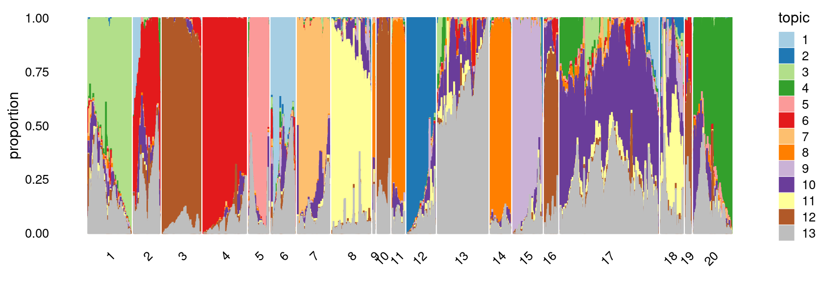
| Version | Author | Date |
|---|---|---|
| a38788b | kevinlkx | 2020-10-20 |
Refine clusters
We then further refine the clusters based on k-means result with \(k = 20\): merge “orange” clusters 9, 11, 14; merge “brown” clusters 3 and 10, 16, 19; merge “yellow” clusters 8 and 18. (maybe could also merge the “red” clusters 2 and 4)
clusters.merged <- clusters.20
clusters.merged[clusters.20 %in% c(9,11,14)] <- 9
clusters.merged[clusters.20 %in% c(3,10,16,19)] <- 3
clusters.merged[clusters.20 %in% c(8,18)] <- 8
clusters.merged <- factor(clusters.merged, labels = paste0("c", c(1:length(unique(clusters.merged)))))
print(sort(table(clusters.merged),decreasing = TRUE))

samples$cluster_kmeans <- clusters.merged
# clusters.merged
#   c13    c3    c8   c11    c4    c1    c9   c14   c10    c7    c2   c12    c5
# 13635  9873  8034  6703  5963  5809  5626  5057  4012  3783  3492  3490  2958
#    c6
#  2738
colors_topics <- c("#a6cee3","#1f78b4","#b2df8a","#33a02c","#fb9a99","#e31a1c",
"#fdbf6f","#ff7f00","#cab2d6","#6a3d9a","#ffff99","#b15928",
"gray")
rows <- sample(nrow(fit$L),4000)
p.structure.5 <- structure_plot(select(poisson2multinom(fit),loadings = rows),
grouping = clusters.merged[rows],n = Inf,gap = 20,
perplexity = 50,topics = 1:13,colors = colors_topics,
num_threads = 4,verbose = FALSE)
# Perplexity automatically changed to 43 because original setting of 50 was too large for the number of samples (134)
# Perplexity automatically changed to 47 because original setting of 50 was too large for the number of samples (147)
print(p.structure.5)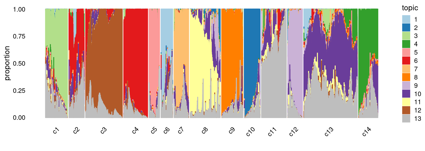
| Version | Author | Date |
|---|---|---|
| a38788b | kevinlkx | 2020-10-20 |
The clusters defined by k-means on topic proportions reasonably identify the clusters shown in the PCA hexbin plots (below).
p.pca.4.1 <- labeled_pca_plot(fit,1:2,samples$cluster_kmeans,font_size = 7,
                       legend_label = "cluster_kmeans")
p.pca.4.2 <- labeled_pca_plot(fit,3:4,samples$cluster_kmeans,font_size = 7,
                       legend_label = "cluster_kmeans")
p.pca.4.3 <- labeled_pca_plot(fit,5:6,samples$cluster_kmeans,font_size = 7,
                       legend_label = "cluster_kmeans")
p.pca.4.4 <- labeled_pca_plot(fit,7:8,samples$cluster_kmeans,font_size = 7,
                       legend_label = "cluster_kmeans")
p.pca.4.5 <- labeled_pca_plot(fit,9:10,samples$cluster_kmeans,font_size = 7,
                       legend_label = "cluster_kmeans")
p.pca.4.6 <- labeled_pca_plot(fit,11:12,samples$cluster_kmeans,font_size = 7,
                       legend_label = "cluster_kmeans")
plot_grid(p.pca.4.1,p.pca.4.2,p.pca.4.3,p.pca.4.4,p.pca.4.5,p.pca.4.6)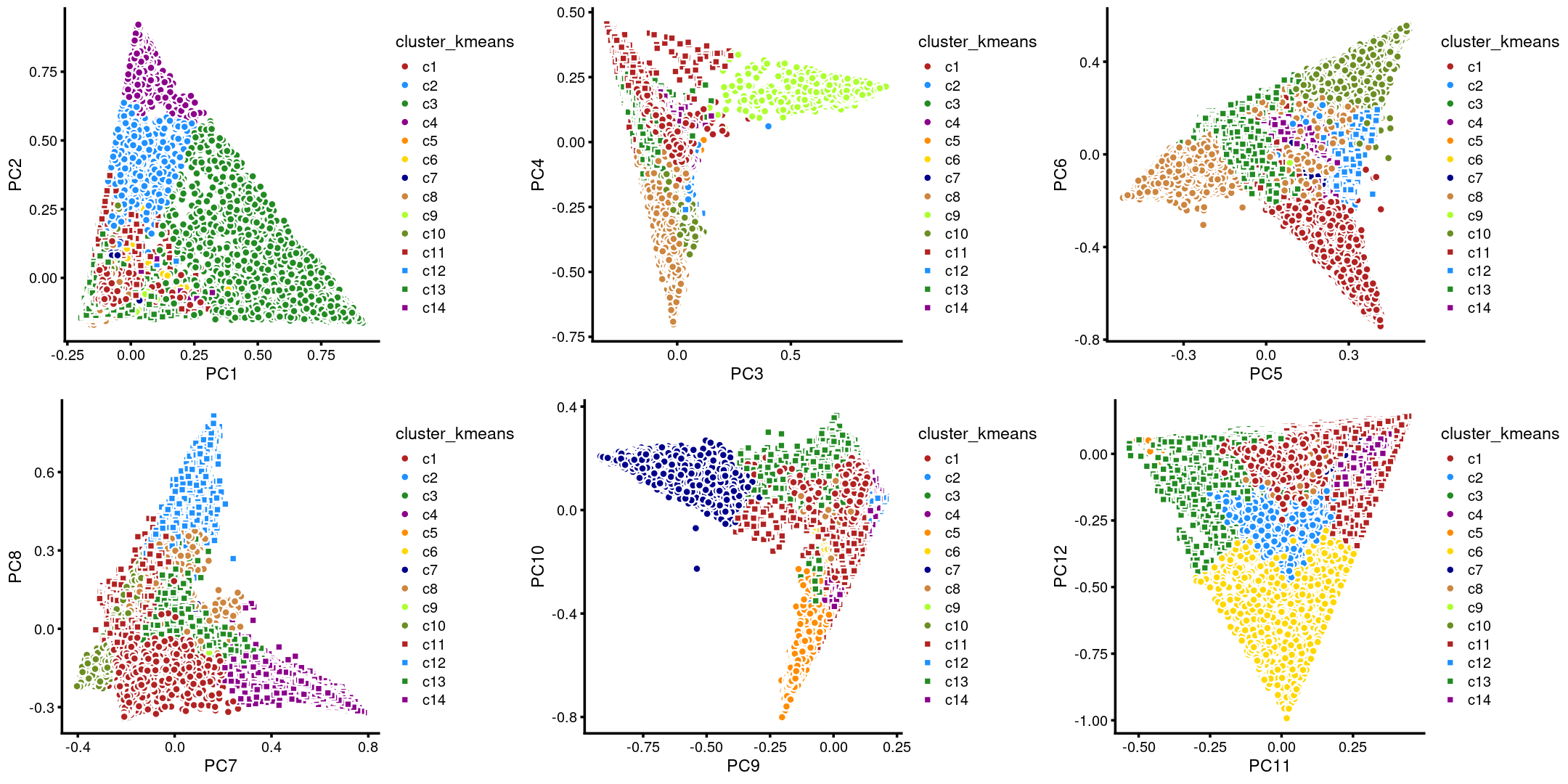
| Version | Author | Date |
|---|---|---|
| a38788b | kevinlkx | 2020-10-20 |
plot_grid(p.pca2.1,p.pca2.2,p.pca2.3,p.pca2.4,p.pca2.5,p.pca2.6)
| Version | Author | Date |
|---|---|---|
| a38788b | kevinlkx | 2020-10-20 |
We then label the cells in each cluster with the known tissue labels.
Tissues:
samples$tissue <- as.factor(samples$tissue)
cat(length(levels(samples$tissue)), "tissues. \n")
table(samples$tissue)
# 13 tissues.
#
#       BoneMarrow       Cerebellum            Heart           Kidney
#             8403             2278             7650             6431
#   LargeIntestine            Liver             Lung PreFrontalCortex
#             7086             6167             9996             5959
#   SmallIntestine           Spleen           Testes           Thymus
#             4077             4020             2723             7617
#       WholeBrain
#             8766
Plot the distribution of tissues by cluster.
Stacked barplot for the counts of tissues by clusters:
library(plyr);library(dplyr)
# ------------------------------------------------------------------------------
# You have loaded plyr after dplyr - this is likely to cause problems.
# If you need functions from both plyr and dplyr, please load plyr first, then dplyr:
# library(plyr); library(dplyr)
# ------------------------------------------------------------------------------
#
# Attaching package: 'plyr'
# The following objects are masked from 'package:dplyr':
#
#     arrange, count, desc, failwith, id, mutate, rename, summarise,
#     summarize
library(RColorBrewer)

freq_cluster_tissue <- count(samples, vars=c("cluster_kmeans","tissue"))

colors_tissues <- colorRampPalette(brewer.pal(9, "Set1"))(13)

# stacked barplot for the counts of tissues by clusters
p.structure.6 <- ggplot(freq_cluster_tissue, aes(fill=tissue, y=freq, x=cluster_kmeans)) +
  geom_bar(position="stack", stat="identity") +
  theme_classic() + xlab("Cluster") + ylab("Number of cells") +
  scale_fill_manual(values = colors_tissues) +
  guides(fill=guide_legend(ncol=2)) +
  theme(
  legend.title = element_text(size = 10),
  legend.text = element_text(size = 8)
  )
print(p.structure.6)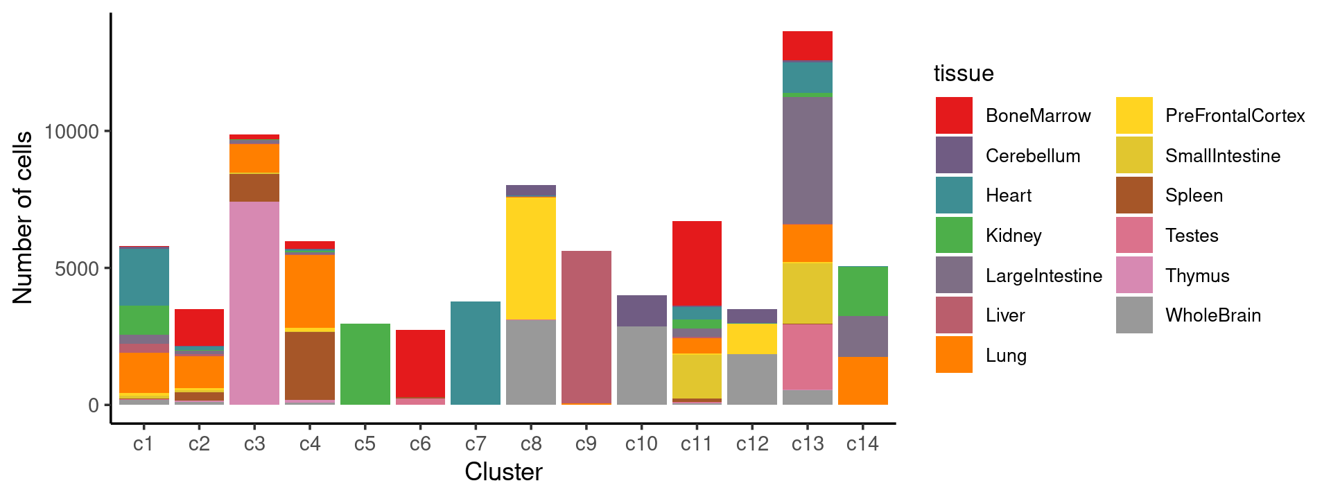
| Version | Author | Date |
|---|---|---|
| b8a48b9 | kevinlkx | 2020-10-20 |
Percent stacked barplot for the counts of tissues by clusters:
freq_cluster_tissue <- count(samples, vars=c("cluster_kmeans","tissue"))

colors_tissues <- colorRampPalette(brewer.pal(9, "Set1"))(13)

p.structure.7 <- ggplot(freq_cluster_tissue, aes(fill=tissue, y=freq, x=cluster_kmeans)) +
  geom_bar(position="fill", stat="identity") +
  theme_classic() + xlab("Cluster") + ylab("Proportion of cells") +
  scale_fill_manual(values = colors_tissues) +
  guides(fill=guide_legend(ncol=2)) +
  theme(
  legend.title = element_text(size = 10),
  legend.text = element_text(size = 8)
  )
print(p.structure.7)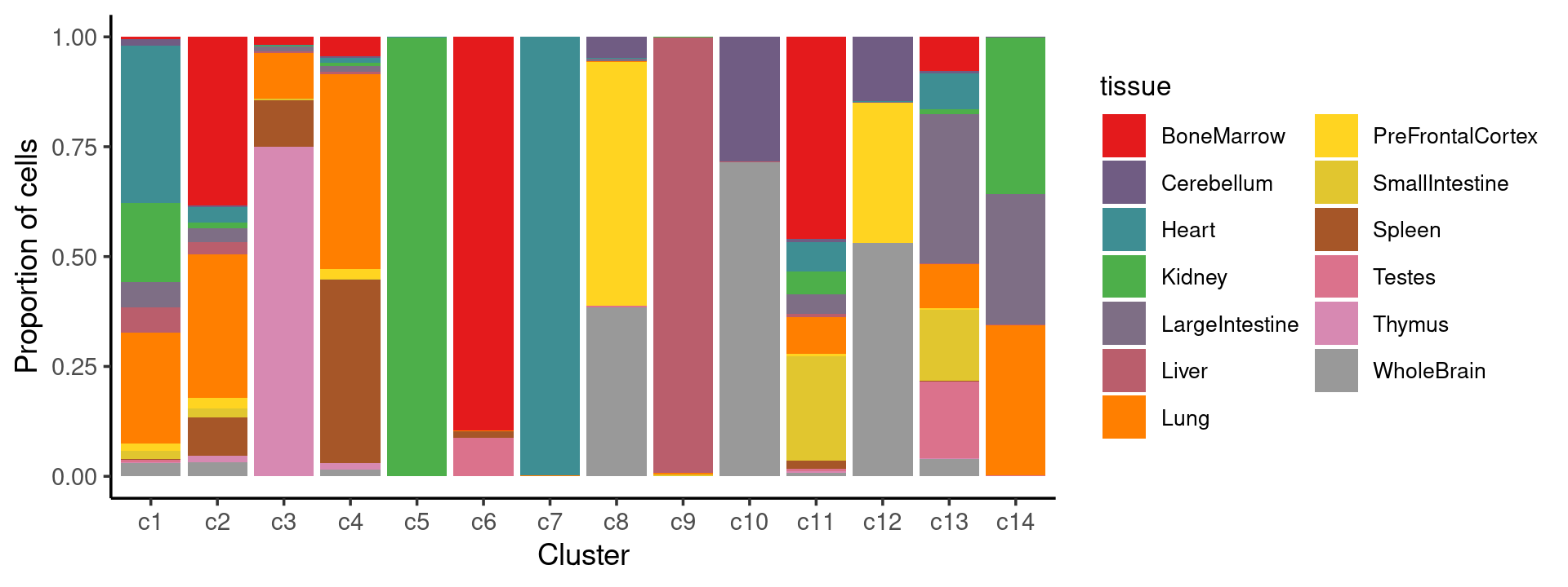
| Version | Author | Date |
|---|---|---|
| b8a48b9 | kevinlkx | 2020-10-20 |
We can see a few clusters are tissue specific: cluster c5 is kidney specific; cluster c7 is heart specific; cluster c9 is liver specific; cluster c3 is primarily thymus; cluster c6 is primarily bone marrow.
Some clusters are combinations of related tissues: cluster c4 is half lung and half spleen; cluster c8 and c12 are mainly from pre-frontal cortex, whole brain (and cerebellum) – all neuron related. cluster c10 is also from whole brain and cerebellum. cluster c14 is mainly from Kidney, LargeIntestine, and Lung.
Some clusters are more heterogeneous mixtures of different tissues: e.g. c1, c2, c11, c13.
freq_cluster_tissue <- with(samples,table(tissue,cluster_kmeans))
print(freq_cluster_tissue)
#                   cluster_kmeans
# tissue               c1   c2   c3   c4   c5   c6   c7   c8   c9  c10  c11  c12
#   BoneMarrow         33 1342  174  259    0 2453    0    1    0    0 3085    0
#   Cerebellum         80    8    0   29    0    0    0  387    0 1140   47  510
#   Heart            2084  128   15   64    5    0 3776   14    0    0  442    4
#   Kidney           1047   45   27   48 2953    0    0    4    3    0  347    1
#   LargeIntestine    328  107  109   70    0    0    1   32    0    0  310    5
#   Liver             334   96   41   36    0    0    0    0 5577    1   47    0
#   Lung             1468 1143 1017 2647    0    2    5   28   28    2  552    2
#   PreFrontalCortex   97   84    1  127    0    0    0 4453    0    2   39 1115
#   SmallIntestine    112   71   49    9    0    0    0    3   15    0 1601    0
#   Spleen              8  302 1033 2498    0   43    0    0    0    0  114    0
#   Testes             34    1    0    2    0  240    0   30    3    0   43    0
#   Thymus              6   56 7406   88    0    0    1    0    0    0   25    0
#   WholeBrain        178  109    1   86    0    0    0 3082    0 2867   51 1853
#                   cluster_kmeans
# tissue              c13  c14
#   BoneMarrow       1056    0
#   Cerebellum         73    4
#   Heart            1113    5
#   Kidney            158 1798
#   LargeIntestine   4617 1507
#   Liver              31    4
#   Lung             1378 1724
#   PreFrontalCortex   38    3
#   SmallIntestine   2212    5
#   Spleen             22    0
#   Testes           2367    3
#   Thymus             31    4
#   WholeBrain        539    0
sessionInfo()
# R version 3.5.1 (2018-07-02)
# Platform: x86_64-pc-linux-gnu (64-bit)
# Running under: Scientific Linux 7.4 (Nitrogen)
#
# Matrix products: default
# BLAS/LAPACK: /software/openblas-0.2.19-el7-x86_64/lib/libopenblas_haswellp-r0.2.19.so
#
# locale:
#  [1] LC_CTYPE=en_US.UTF-8       LC_NUMERIC=C
#  [3] LC_TIME=en_US.UTF-8        LC_COLLATE=en_US.UTF-8
#  [5] LC_MONETARY=en_US.UTF-8    LC_MESSAGES=en_US.UTF-8
#  [7] LC_PAPER=en_US.UTF-8       LC_NAME=C
#  [9] LC_ADDRESS=C               LC_TELEPHONE=C
# [11] LC_MEASUREMENT=en_US.UTF-8 LC_IDENTIFICATION=C
#
# attached base packages:
# [1] stats     graphics  grDevices utils     datasets  methods   base
#
# other attached packages:
# [1] RColorBrewer_1.1-2 plyr_1.8.6         fastTopics_0.3-180 cowplot_1.0.0
# [5] ggplot2_3.3.0      dplyr_0.8.5        Matrix_1.2-15      workflowr_1.6.2
#
# loaded via a namespace (and not attached):
#  [1] ggrepel_0.8.2      Rcpp_1.0.4.6       lattice_0.20-38    tidyr_0.8.3
#  [5] prettyunits_1.1.1  assertthat_0.2.1   rprojroot_1.3-2    digest_0.6.25
#  [9] R6_2.4.1           backports_1.1.7    MatrixModels_0.4-1 evaluate_0.14
# [13] coda_0.19-2        httr_1.4.1         pillar_1.4.4       rlang_0.4.6
# [17] progress_1.2.2     lazyeval_0.2.2     data.table_1.12.8  irlba_2.3.3
# [21] SparseM_1.77       whisker_0.4        hexbin_1.28.1      rmarkdown_2.1
# [25] labeling_0.3       Rtsne_0.15         stringr_1.4.0      htmlwidgets_1.5.1
# [29] munsell_0.5.0      compiler_3.5.1     httpuv_1.5.3.1     xfun_0.14
# [33] pkgconfig_2.0.3    mcmc_0.9-7         htmltools_0.4.0    tidyselect_0.2.5
# [37] tibble_3.0.1       quadprog_1.5-5     viridisLite_0.3.0  crayon_1.3.4
# [41] withr_2.1.2        later_1.0.0        MASS_7.3-51.6      grid_3.5.1
# [45] jsonlite_1.6       gtable_0.3.0       lifecycle_0.2.0    git2r_0.27.1
# [49] magrittr_1.5       scales_1.1.1       RcppParallel_4.4.3 stringi_1.4.6
# [53] farver_2.0.3       fs_1.3.1           promises_1.1.0     ellipsis_0.3.1
# [57] vctrs_0.3.0        tools_3.5.1        glue_1.4.1         purrr_0.3.4
# [61] hms_0.4.2          yaml_2.2.0         colorspace_1.4-1   plotly_4.8.0
# [65] knitr_1.28         quantreg_5.36      MCMCpack_1.4-4