Motif analysis using topic modeling results for Buenrostro et al (2018) scATAC-seq result (data processed using Chen 2019 pipeline)
Kaixuan Luo
Last updated: 2021-02-01
Checks: 7 0
Knit directory: scATACseq-topics/
This reproducible R Markdown analysis was created with workflowr (version 1.6.2). The Checks tab describes the reproducibility checks that were applied when the results were created. The Past versions tab lists the development history.
Great! Since the R Markdown file has been committed to the Git repository, you know the exact version of the code that produced these results.
Great job! The global environment was empty. Objects defined in the global environment can affect the analysis in your R Markdown file in unknown ways. For reproduciblity it's best to always run the code in an empty environment.
The command set.seed(20200729) was run prior to running the code in the R Markdown file. Setting a seed ensures that any results that rely on randomness, e.g. subsampling or permutations, are reproducible.
Great job! Recording the operating system, R version, and package versions is critical for reproducibility.
Nice! There were no cached chunks for this analysis, so you can be confident that you successfully produced the results during this run.
Great job! Using relative paths to the files within your workflowr project makes it easier to run your code on other machines.
Great! You are using Git for version control. Tracking code development and connecting the code version to the results is critical for reproducibility.
The results in this page were generated with repository version 554f088. See the Past versions tab to see a history of the changes made to the R Markdown and HTML files.
Note that you need to be careful to ensure that all relevant files for the analysis have been committed to Git prior to generating the results (you can use wflow_publish or wflow_git_commit). workflowr only checks the R Markdown file, but you know if there are other scripts or data files that it depends on. Below is the status of the Git repository when the results were generated:
Ignored files:
    Ignored:    .Rhistory
    Ignored:    .Rproj.user/

Untracked files:
    Untracked:  analysis/gene_analysis_Buenrostro2018_Chen2019pipeline.Rmd
    Untracked:  analysis/process_data_Buenrostro2018_Chen2019.Rmd
    Untracked:  output/clustering-Cusanovich2018.rds
    Untracked:  scripts/fit_all_models_Buenrostro_2018_chromVar_scPeaks_filtered.sbatch
    Untracked:  scripts/fit_models_Cusanovich2018_tissues.sh

Unstaged changes:
    Modified:   scripts/fit_poisson_nmf.sbatch
    Modified:   scripts/prefit_poisson_nmf.sbatch
Note that any generated files, e.g. HTML, png, CSS, etc., are not included in this status report because it is ok for generated content to have uncommitted changes.
These are the previous versions of the repository in which changes were made to the R Markdown (analysis/motif_analysis_Buenrostro2018_Chen2019pipeline.Rmd) and HTML (docs/motif_analysis_Buenrostro2018_Chen2019pipeline.html) files. If you've configured a remote Git repository (see ?wflow_git_remote), click on the hyperlinks in the table below to view the files as they were in that past version.
| File | Version | Author | Date | Message |
|---|---|---|---|---|
| Rmd | 554f088 | kevinlkx | 2021-02-01 | minor change on figure and font size |
| html | 0fec792 | kevinlkx | 2021-02-01 | Build site. |
| Rmd | 4e6a0b0 | kevinlkx | 2021-02-01 | updated motif heatmaps and motif-gene correlation scatterplots |
| html | 45cb9a0 | kevinlkx | 2021-01-28 | Build site. |
| Rmd | c1f6331 | kevinlkx | 2021-01-28 | change the example volcano plot to topic 4 |
| html | c7742f0 | kevinlkx | 2021-01-28 | Build site. |
| Rmd | 3608c72 | kevinlkx | 2021-01-28 | motif analysis of Buenrostro2018 data with topic 4 examples |
Here we perform TF motif analysis for the Buenrostro et al (2018) scATAC-seq result inferred from the multinomial topic model with \(k = 11\).
We use binarized scPeaks and scATAC-seq data was processed using Chen et al (2019) pipeline.
Load packages and some functions used in this analysis
library(Matrix)
library(fastTopics)
library(dplyr)
library(tidyr)
library(ggplot2)
library(ggrepel)
library(cowplot)
library(plotly)
library(htmlwidgets)
library(DT)
library(reshape2)
library(Logolas)
library(grid)
source("code/motif_analysis.R")
source("code/plots.R")
Load data and topic model results
Load the binarized data and the \(k = 11\) Poisson NMF fit results
data.dir <- "/project2/mstephens/kevinluo/scATACseq-topics/data/Buenrostro_2018/processed_data_Chen2019pipeline/"
load(file.path(data.dir, "Buenrostro_2018_binarized_counts.RData"))
cat(sprintf("%d x %d counts matrix.\n",nrow(counts),ncol(counts)))
# 2034 x 101172 counts matrix.fit.dir <- "/project2/mstephens/kevinluo/scATACseq-topics/output/Buenrostro_2018_Chen2019pipeline/binarized/"
fit <- readRDS(file.path(fit.dir, "/fit-Buenrostro2018-binarized-scd-ex-k=11.rds"))$fit
fit_multinom <- poisson2multinom(fit)Visualize by Structure plot grouped by cell labels.
set.seed(10)
colors_topics <- c("#a6cee3","#1f78b4","#b2df8a","#33a02c","#fb9a99","#e31a1c",
                   "#fdbf6f","#ff7f00","#cab2d6","#6a3d9a","#ffff99","#b15928",
                   "gray")
samples$label <- factor(samples$label, levels = c("HSC", "MPP", "CMP", "GMP", "mono", "MEP", "LMPP", "CLP", "pDC", "UNK"))

p.structure <- structure_plot(fit_multinom,
                     grouping = samples[, "label"],n = Inf,gap = 40,
                     perplexity = 50,topics = 1:11,colors = colors_topics,
                     num_threads = 4,verbose = FALSE)

print(p.structure)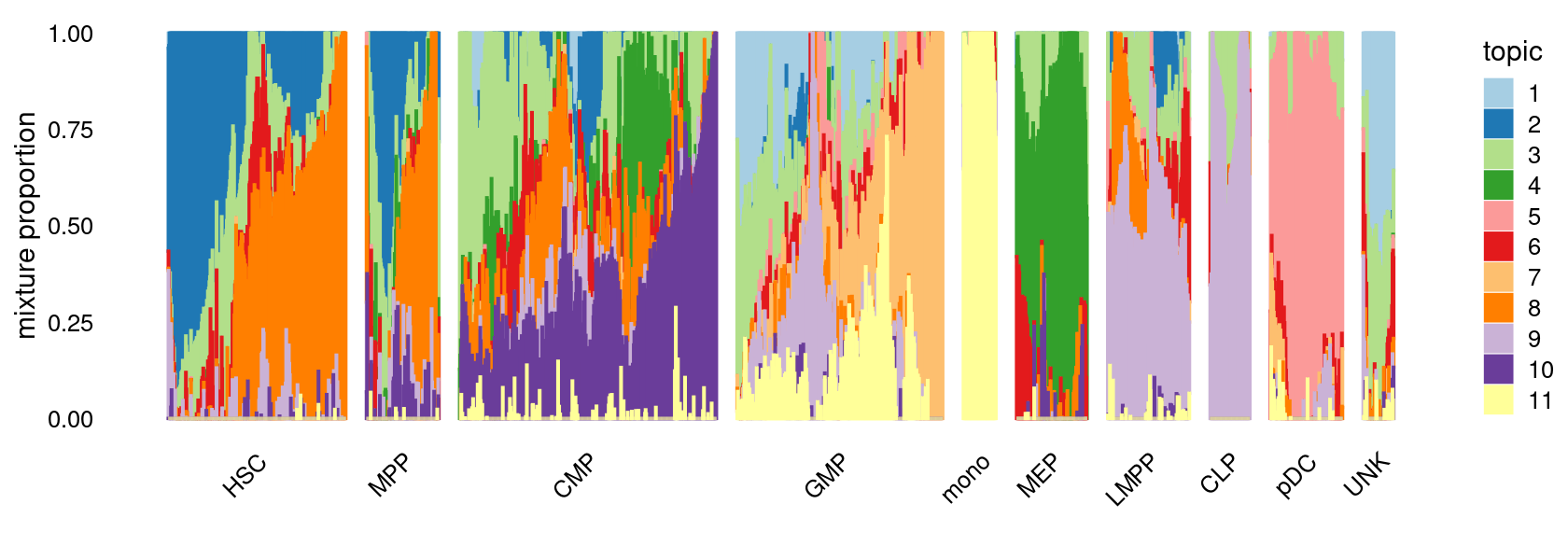
Heatmap of average mixture proportions by cell labels.
create_celllabel_topic_heatmap(fit_multinom, grouping = samples[, "label"], cluster_topics = FALSE,
                               group_labels = c("HSC", "MPP", "CMP", "MEP", "LMPP", "GMP", "mono", "pDC", "CLP", "UNK"))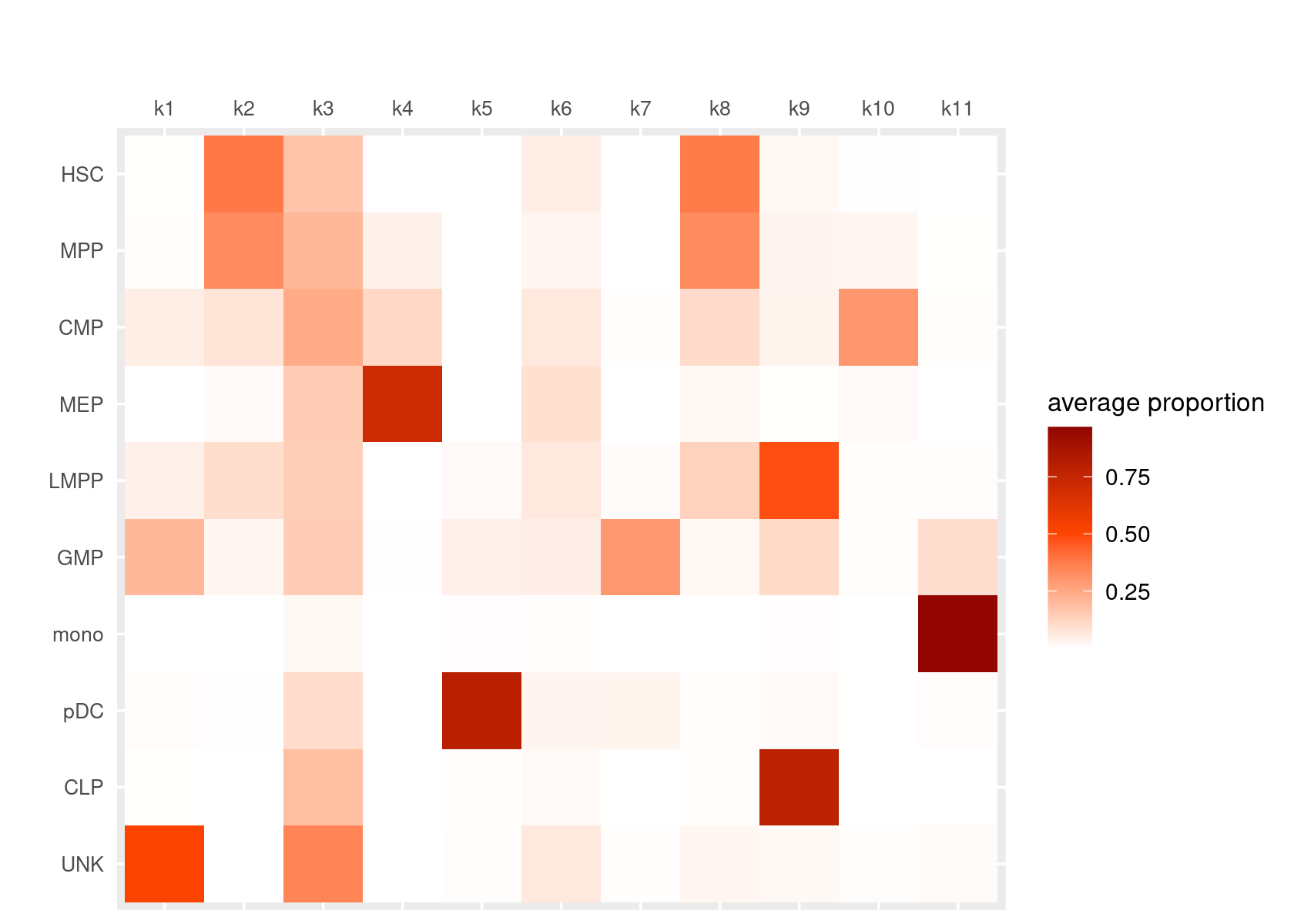
| Version | Author | Date |
|---|---|---|
| 0fec792 | kevinlkx | 2021-02-01 |
Focus on myeloid differentiation (HSC, CMP, GMP, Momo)
set.seed(10)
colors_topics <- c("#a6cee3","#1f78b4","#b2df8a","#33a02c","#fb9a99","#e31a1c",
                   "#fdbf6f","#ff7f00","#cab2d6","#6a3d9a","#ffff99","#b15928",
                   "gray")
myeloid_samples <- factor(samples$label, levels = c("HSC", "MPP", "CMP", "GMP", "mono"))

p.structure.myeloid <- structure_plot(fit_multinom,
                     grouping = myeloid_samples, n = Inf,gap = 40,
                     perplexity = 50,topics = 1:11,colors = colors_topics,
                     num_threads = 4,verbose = FALSE)

print(p.structure.myeloid)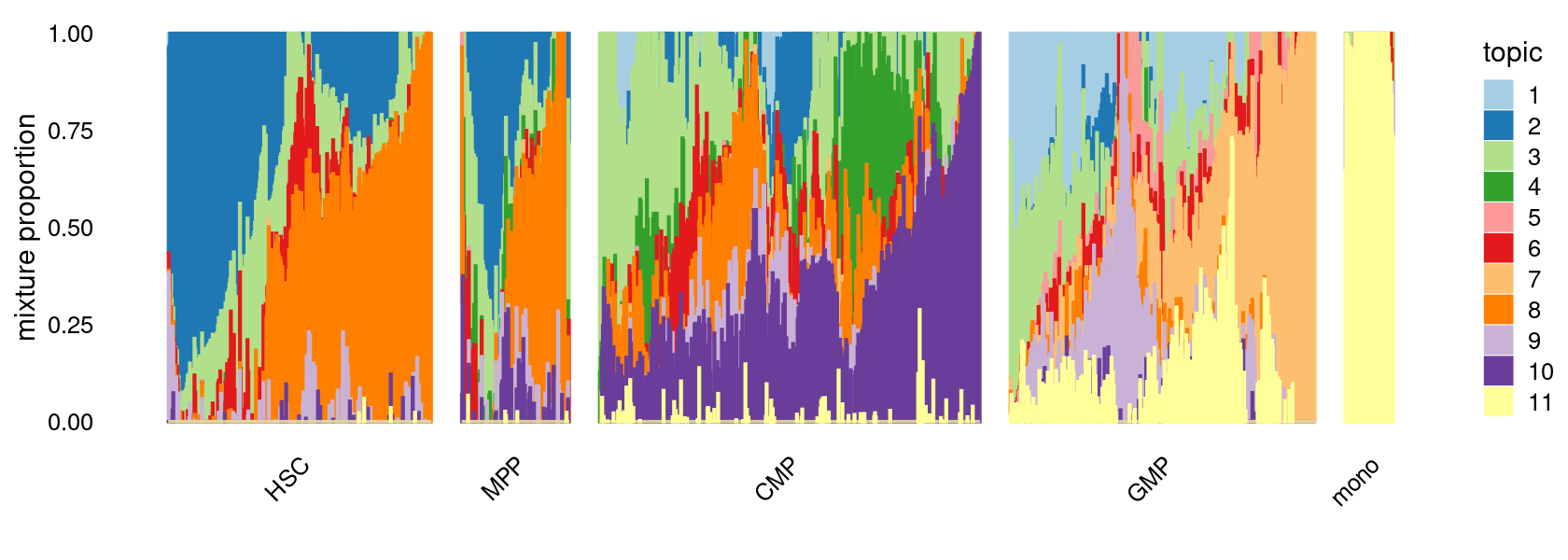
| Version | Author | Date |
|---|---|---|
| 0fec792 | kevinlkx | 2021-02-01 |
Differential accessbility analysis of the ATAC-seq regions for the topics
Load results from differential accessbility analysis for the topics
out.dir <- "/project2/mstephens/kevinluo/scATACseq-topics/output/Buenrostro_2018_Chen2019pipeline/binarized/"
cat(sprintf("Load results from %s \n", out.dir))
# Load results from /project2/mstephens/kevinluo/scATACseq-topics/output/Buenrostro_2018_Chen2019pipeline/binarized/diff_count_topics <- readRDS(file.path(out.dir, "diffcount-Buenrostro2018-11topics.rds"))Distribution of z-scores
zscore_topics <-  melt(diff_count_topics$Z)
colnames(zscore_topics) <- c("region", "topic", "zscore")
levels(zscore_topics$topic) <- colnames(diff_count_topics$Z)

z.quantile.99 <- apply(abs(diff_count_topics$Z), 2, quantile, 0.99)
cat("z-score 99% quantile: \n")
print(z.quantile.99)

p.hist.zscores <- ggplot(zscore_topics, aes(x=zscore)) +
  geom_histogram(binwidth=1, color="black", fill="white") +
  coord_cartesian(xlim = c(-10, 30)) + theme_cowplot(font_size = 10) +
  facet_wrap(~ topic, ncol=4)

print(p.hist.zscores)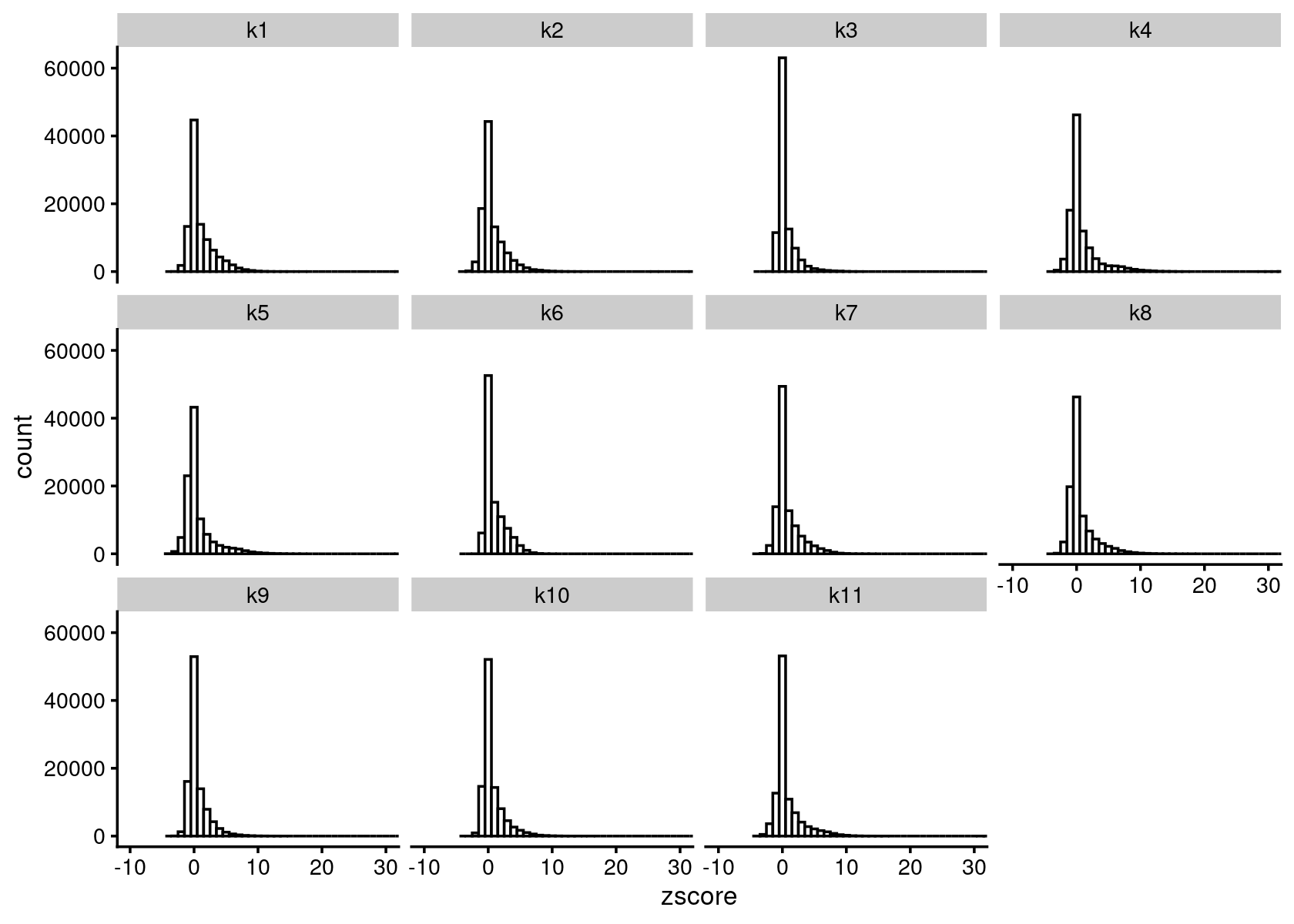
| Version | Author | Date |
|---|---|---|
| c7742f0 | kevinlkx | 2021-01-28 |
# z-score 99% quantile:
#        k1        k2        k3        k4        k5        k6        k7        k8
#  7.680613  7.226323  5.954049 10.059326  9.203917  5.821598  7.215842  8.156498
#        k9       k10       k11
#  5.978363  6.684635  8.191629
Volcano plot of the regions
topic 1 and topic 4 examples
p.volcano.1 <- volcano_plot(diff_count_topics,k = 1,label_above_quantile = Inf,
             subsample_below_quantile = 0.7, subsample_rate = 0.1)
# 37434 out of 101172 data points will be included in plotp.volcano.4 <- volcano_plot(diff_count_topics,k = 4,label_above_quantile = Inf,
subsample_below_quantile = 0.7, subsample_rate = 0.1)# 37434 out of 101172 data points will be included in plotplot_grid(p.volcano.1, p.volcano.4)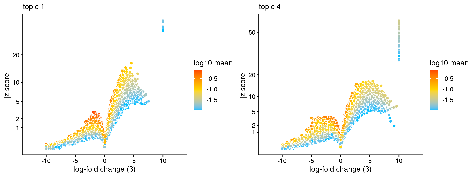
Motif enrichment analysis using HOMER
- Details about HOMER motif analysis:
- Motif enrichment result using regions with z-score above 99% quantile.
Compile Homer results across topics
homer.dir <- paste0(out.dir, "/motifanalysis-Buenrostro2018-k=11-quantile/HOMER/")
cat(sprintf("Directory of motif analysis result: %s \n", homer.dir))
homer_res_topics <- readRDS(file.path(homer.dir, "/homer_knownResults.rds"))
selected_regions <- readRDS(file.path(homer.dir, "/selected_regions.rds"))

# Compile Homer results (pvalue and ranking) across topics
motif_res <- compile_homer_motif_res(homer_res_topics)
saveRDS(motif_res, paste0(homer.dir, "/homer_motif_enrichment_results.rds"))
cat("compiled homer motif results are saved in", paste0(homer.dir, "/homer_motif_enrichment_results.rds \n"))

motif_table <- data.frame(motif = gsub("/.*", "", rownames(motif_res$mlog10P)),
                          round(motif_res$mlog10P,2))
DT::datatable(motif_table, rownames = F, caption = "Motif enrichment (-log10P)")
# Directory of motif analysis result: /project2/mstephens/kevinluo/scATACseq-topics/output/Buenrostro_2018_Chen2019pipeline/binarized//motifanalysis-Buenrostro2018-k=11-quantile/HOMER/
# compiled homer motif results are saved in /project2/mstephens/kevinluo/scATACseq-topics/output/Buenrostro_2018_Chen2019pipeline/binarized//motifanalysis-Buenrostro2018-k=11-quantile/HOMER//homer_motif_enrichment_results.rdsTop 10 motifs in each topic
cat("Number of regions selected for each topic: \n")
print(mapply(nrow, selected_regions[1:(length(selected_regions)-1)]))

colnames_homer <- c("motif_name", "consensus", "P", "log10P", "Padj",  "num_target", "percent_target", "num_bg", "percent_bg")

top_motifs <- data.frame(matrix(nrow=10, ncol = length(homer_res_topics)))
colnames(top_motifs) <- names(homer_res_topics)
for (k in 1:length(homer_res_topics)){
  homer_res <- homer_res_topics[[k]]
  colnames(homer_res) <- colnames_homer
  homer_res <- homer_res %>% separate(motif_name, c("motif", "origin", "database"), "/")
  top_motifs[,k] <- head(homer_res$motif, 10)
}

DT::datatable(data.frame(rank = 1:10, top_motifs), rownames = F, caption = "Top 10 motifs enriched in each topic.")
# Number of regions selected for each topic:
# k1 k2 k3 k4 k5 k6 k7 k8 k9 k10 k11
# 1012 1012 1012 1012 1012 1012 1012 1012 1012 1012 1012Heatmap of motif enrichment across topics
Heatmap of motif enrichment -log10(p-value). Order motifs by hierarchical clustering.
create_motif_enrichment_heatmap(motif_res, enrichment = "-log10(p-value)",
                                cluster_motifs = TRUE, cluster_topics = TRUE, motif_filter = 10, horizontal = FALSE,
                                enrichment_range = c(0,100), method_cluster = "average", font.size.motifs = 4, font.size.topics = 9)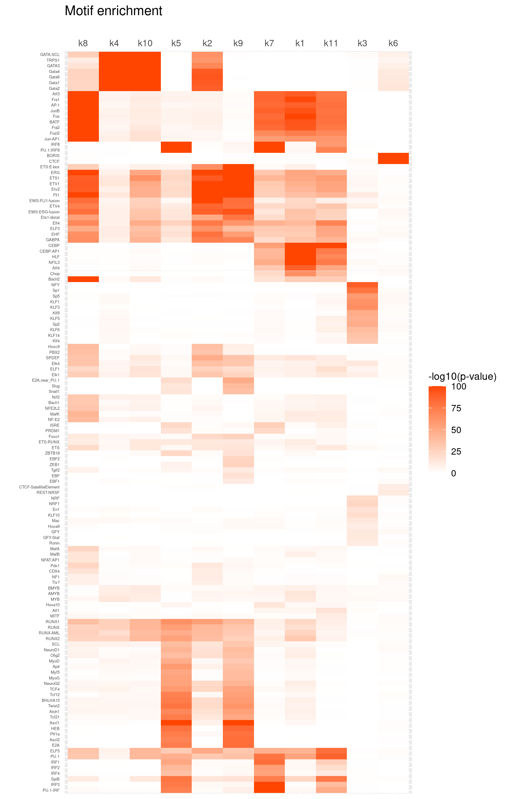
# 132 out of 439 motifs included the heatmapHeatmap of motif enrichment z-score. Order motifs by hierarchical clustering.
create_motif_enrichment_heatmap(motif_res, enrichment = "z-score",
                                cluster_motifs = TRUE, cluster_topics = FALSE, motif_filter = 10, horizontal = FALSE,
                                enrichment_range = c(-20,20), method_cluster = "average", font.size.motifs = 4, font.size.topics = 9)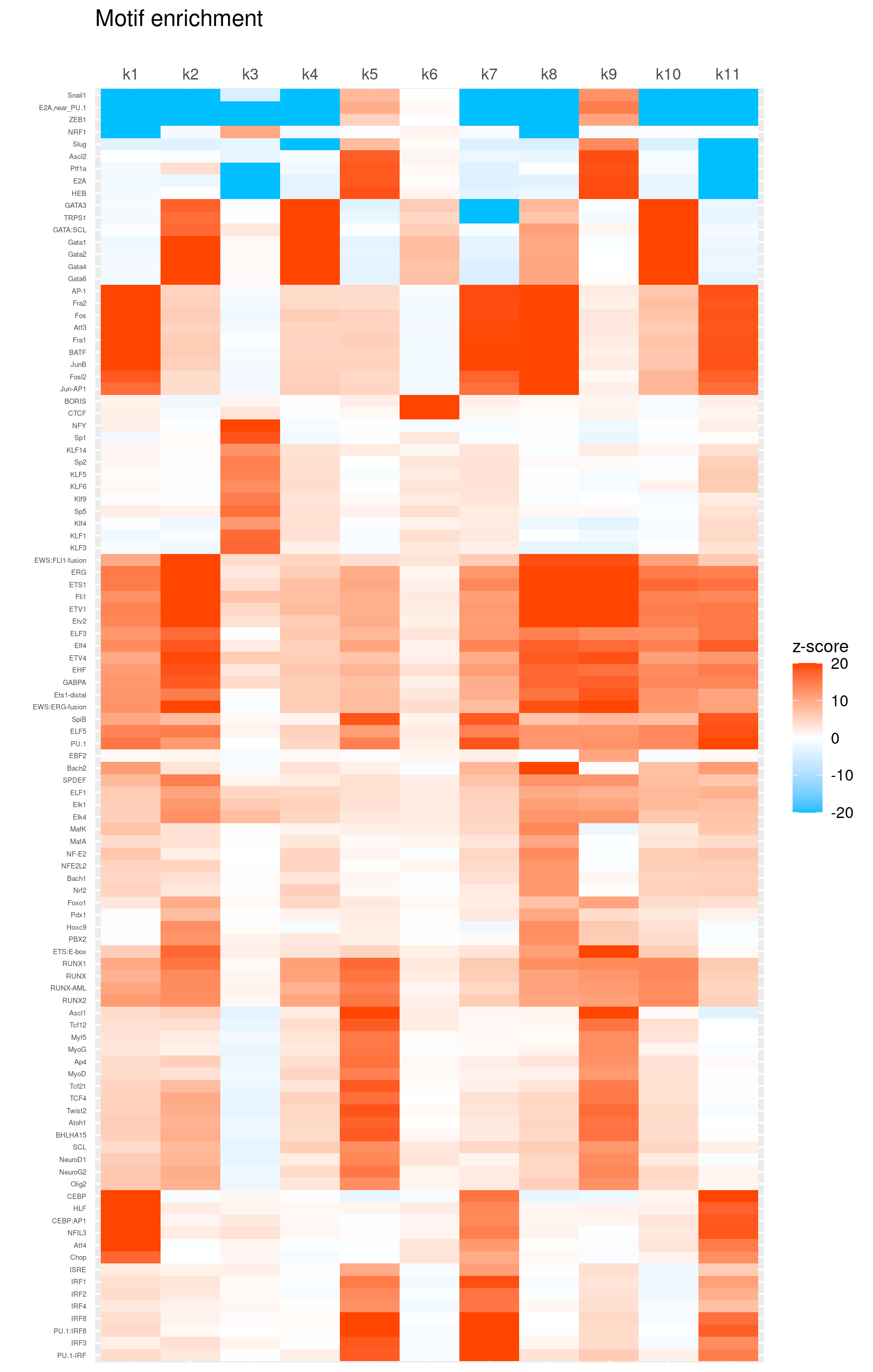
# 104 out of 439 motifs included the heatmapHeatmap of motif enrichment for selected TF motifs
toMatch <- c("^GATA\\d*$", "^CEBP.?$", "^SPI.?$", "^IRF\\d*$", "^STAT\\d*$", "^TCF\\d*$", "^BCL\\d*$", "^CTCF$", "^ERG$")
selected_motifs <- grep(paste(toMatch,collapse="|"), motif_res$motifs$motif, ignore.case = T, value = T)
rows <- match(selected_motifs, motif_res$motifs$motif)
selected_motif_res <- lapply(motif_res, FUN = function(x) {x[rows, ]})
Heatmap of motif enrichment -log10(p-value). Order motifs by hierarchical clustering.
create_motif_enrichment_heatmap(selected_motif_res, enrichment = "-log10(p-value)",
                                cluster_motifs = TRUE, cluster_topics = TRUE, motif_filter = 10, horizontal = FALSE,
                                enrichment_range = c(0,100), method_cluster = "average",  font.size.motifs = 8, font.size.topics = 9)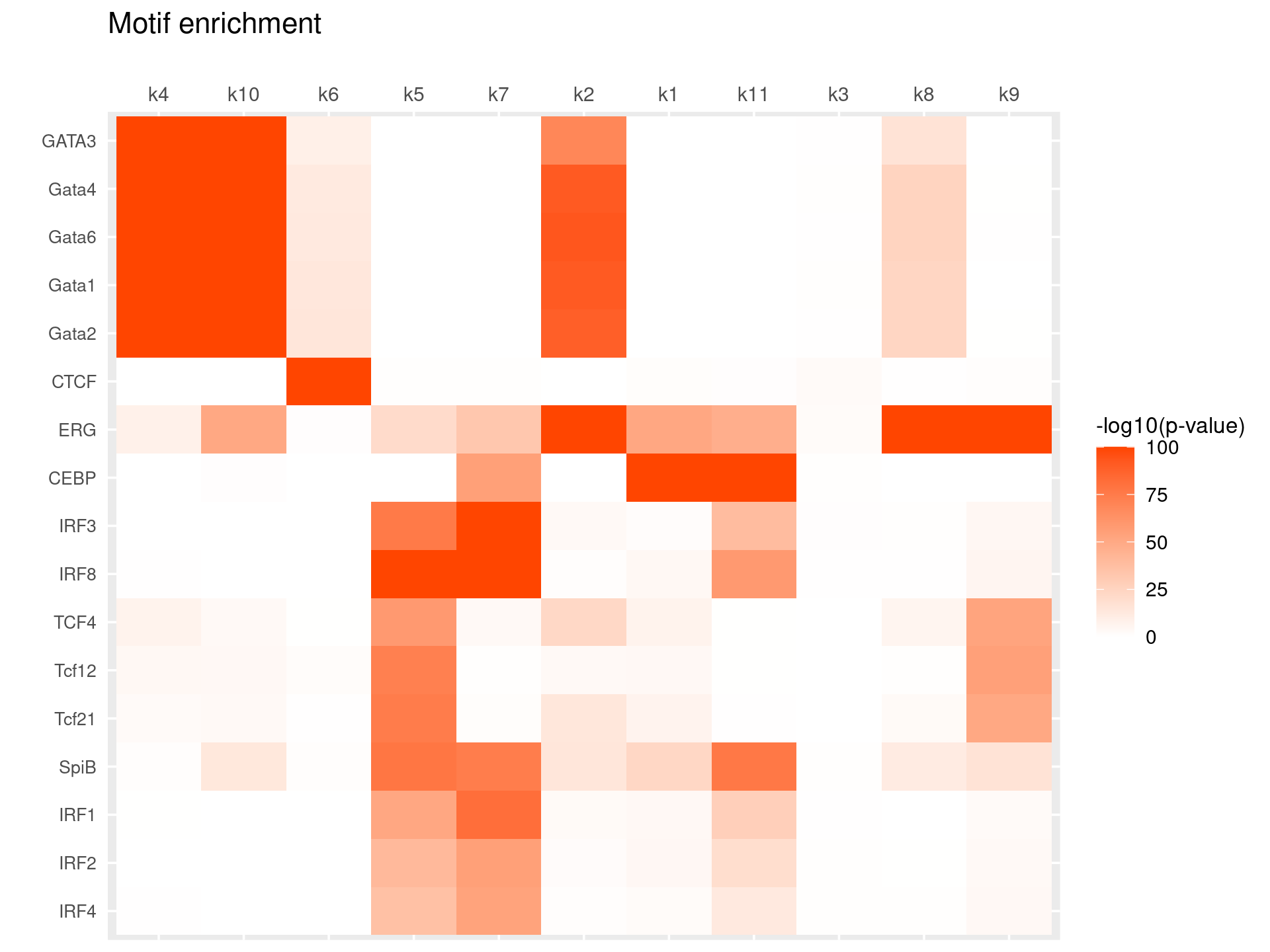
| Version | Author | Date |
|---|---|---|
| 0fec792 | kevinlkx | 2021-02-01 |
# 17 out of 26 motifs included the heatmapHeatmap of motif enrichment z-score. Order motifs by hierarchical clustering.
create_motif_enrichment_heatmap(selected_motif_res, enrichment = "z-score",
                                cluster_motifs = TRUE, cluster_topics = FALSE, motif_filter = 10, horizontal = FALSE,
                                enrichment_range = c(-20,20), method_cluster = "average", font.size.motifs = 8, font.size.topics = 9)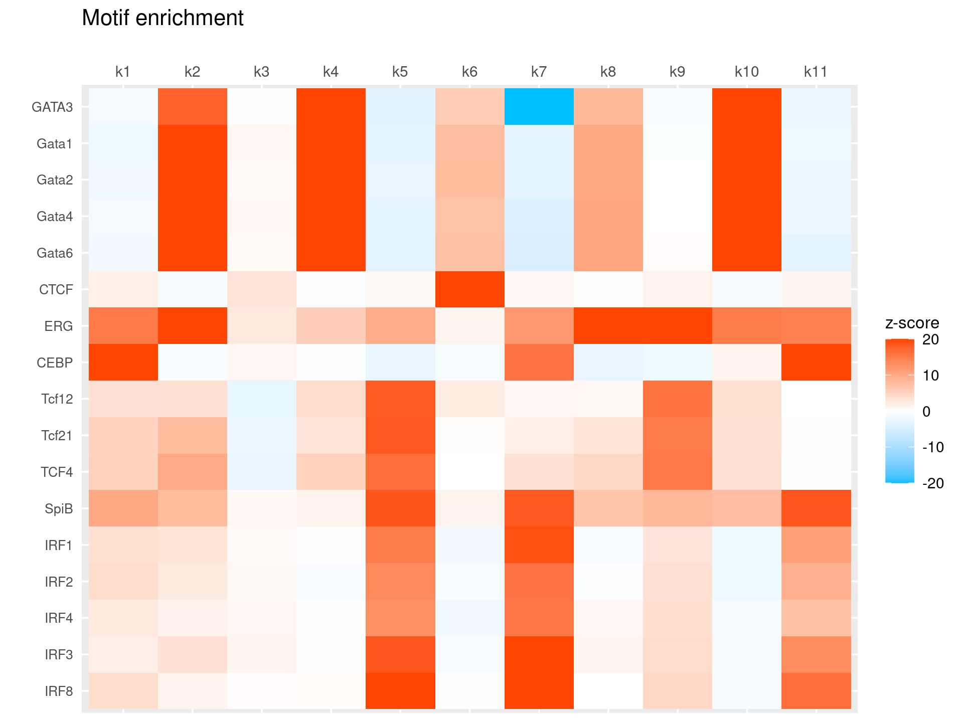
| Version | Author | Date |
|---|---|---|
| 0fec792 | kevinlkx | 2021-02-01 |
# 17 out of 26 motifs included the heatmapScatterplots of motif enrichment
Plot motif enrichment (-log10 p-value) and the ranking
# Plot enrichment (-log10 p-value) and ranking of the motifs

plots <- vector("list", ncol(motif_res$mlog10P))
names(plots) <- colnames(motif_res$mlog10P)

for( i in 1:length(plots)){
  plots[[i]] <- create_motif_enrichment_ranking_plot(motif_res, k = i,
                                                     max.overlaps = 20, subsample = FALSE)
}

do.call(plot_grid,plots)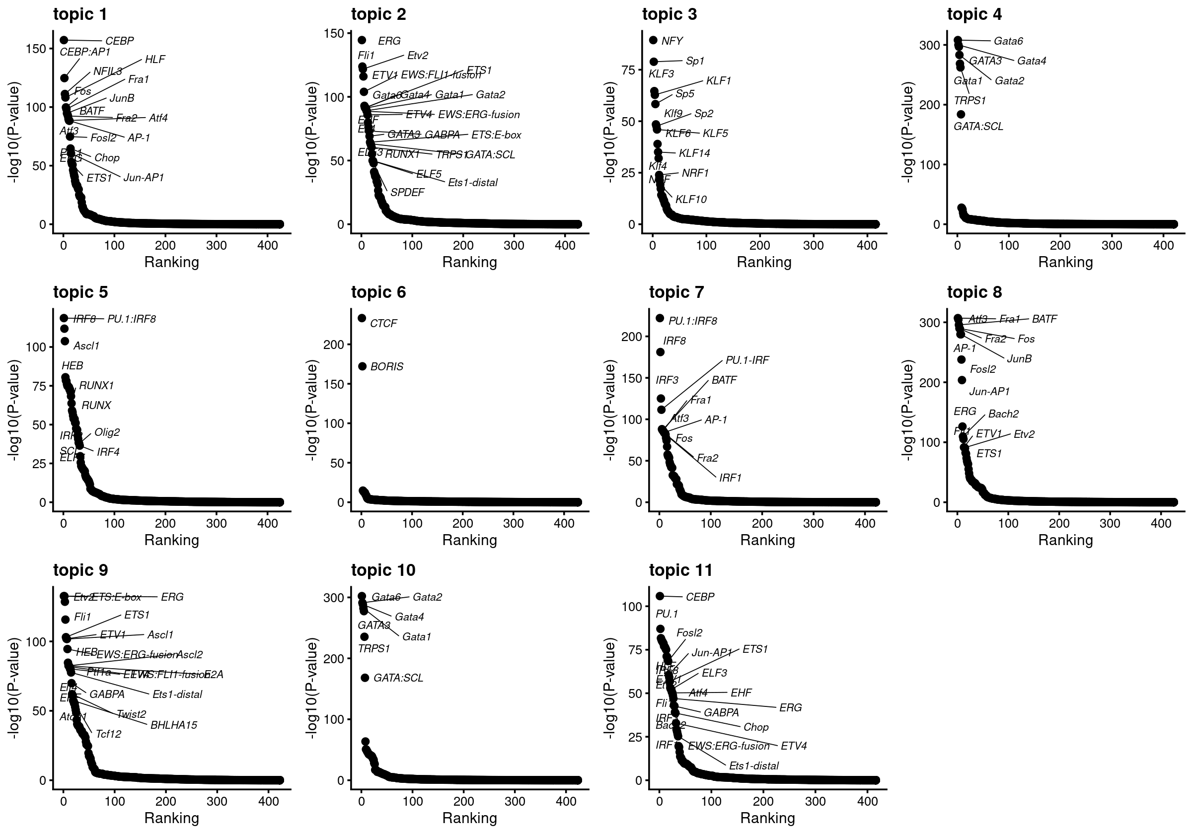
| Version | Author | Date |
|---|---|---|
| 0fec792 | kevinlkx | 2021-02-01 |
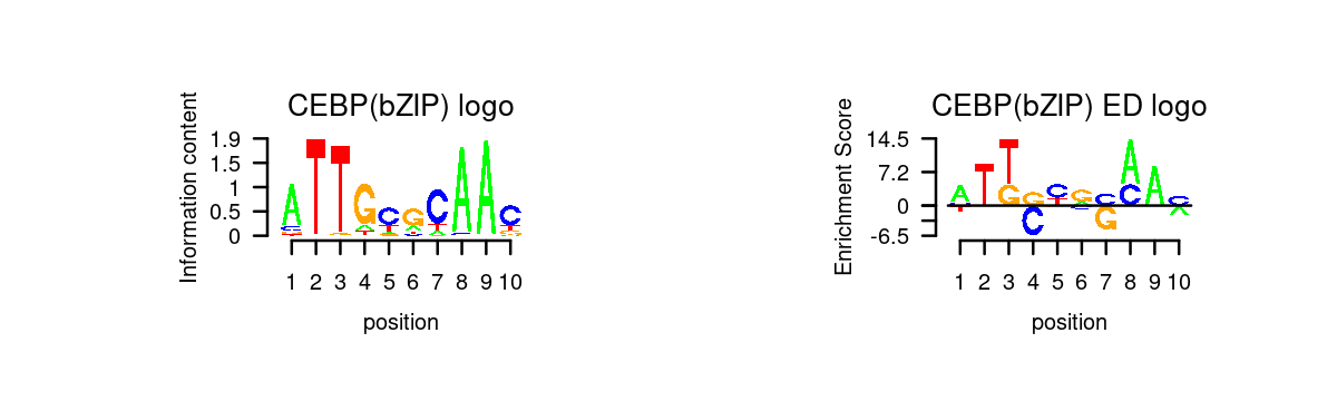
Examples Topic 1 is mainly shown in GMP. The enrichment of CEBP motif in GMP is also highlighted in Figure 2F of the Buenrostro et al paper.
Topic 4 is mainly shown in MEP especially and also CMP. The enrichment of GATA motif in MEP and CMP is also highlighted in Figure 2E of the Buenrostro et al paper.
do.call(plot_grid,plots[c(1,4)])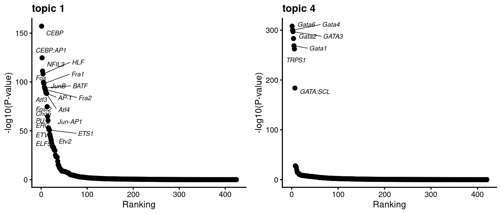
# Plot motif enrichment (-log10 p-value) in each topic vs other topics

plots <- vector("list", ncol(motif_res$mlog10P))
names(plots) <- colnames(motif_res$mlog10P)

for( i in 1:length(homer_res_topics)){
  plots[[i]] <- create_motif_enrichment_plot(motif_res, k = i,
                                             max.overlaps = 20, subsample = TRUE)
}

do.call(plot_grid,plots)
Motif enrichment vs gene score
Load pre-computed gene scores
gene.dir <- paste0(out.dir, "/geneanalysis-Buenrostro2018-k=11-TSS-l2")
cat(sprintf("Directory of gene analysis result: %s \n", gene.dir))
genescore_res <- readRDS(file.path(gene.dir, "genescore_result_topics.rds"))
# Directory of gene analysis result: /project2/mstephens/kevinluo/scATACseq-topics/output/Buenrostro_2018_Chen2019pipeline/binarized//geneanalysis-Buenrostro2018-k=11-TSS-l2Get TF genes
motif_names <- motif_res$motifs$motif
gene_names <- genescore_res$genes$SYMBOL
common_genes <- intersect(toupper(motif_names), toupper(gene_names))
cat(sprintf("%s TF genes mapped between motif names and gene symbol. \n", length(common_genes)))

motif_gene_table <- data.frame(motif = motif_names[match(common_genes, toupper(motif_names))],
                                      gene = gene_names[match(common_genes, toupper(gene_names))])
# 263 TF genes mapped between motif names and gene symbol.Compute correlation between motif enrichment z-score and gene score:
Topic 4 example
- Compute motif enrichment z-scores from the motif enrichment p-values
- Plot motif enrichment (-log10 p-value) and correlation between motif enrichment z-scores and gene scores
- Rank motifs by motif enrichment (-log10 p-value) and correlation between motif enrichment z-score and gene scores
motif_gene_mapping <- create_motif_gene_cor_scatterplot(motif_res, genescore_res, motif_gene_table,
                                                        k = 4, cor.motif = "z-score")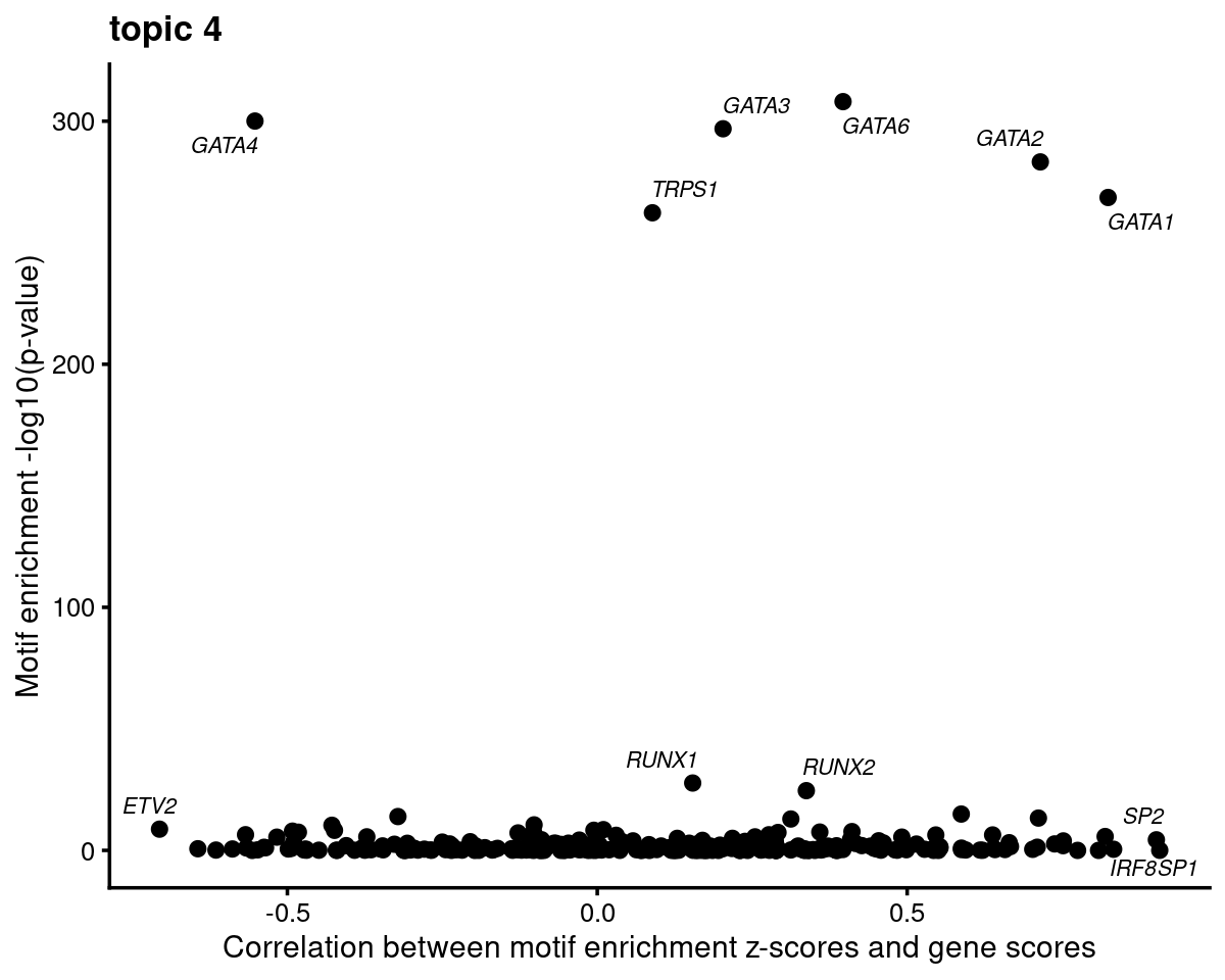
motif_gene_mapping <- motif_gene_mapping[with(motif_gene_mapping, order(motif_mlog10P*cor_zscore, decreasing = T)),]
rownames(motif_gene_mapping) <- 1:nrow(motif_gene_mapping)

cat("Top 10 motifs by motif enrichment (-log10 p-value) and correlation to gene scores: \n")
print(head(motif_gene_mapping[,c("motif","motif_mlog10P", "gene_score", "cor_zscore")], 10))
# Top 10 motifs by motif enrichment (-log10 p-value) and correlation to gene scores:
# motif motif_mlog10P gene_score cor_zscore
# 1 Gata1(Zf) 268.611137 10.58850478 0.82417385
# 2 Gata2(Zf) 283.246861 3.50532676 0.71486568
# 3 Gata6(Zf) 308.045076 0.28569100 0.39652411
# 4 GATA3(Zf) 296.883708 0.44378118 0.20293328
# 5 TRPS1(Zf) 262.313867 0.18883601 0.08901704
# 6 Fli1(ETS) 13.293754 -0.02447725 0.71178359
# 7 ETV1(ETS) 14.944073 -0.85762399 0.58726309
# 8 RUNX2(Runt) 24.572382 -1.08635191 0.33730209
# 9 Foxo1(Forkhead) 5.706629 3.14525125 0.81941673
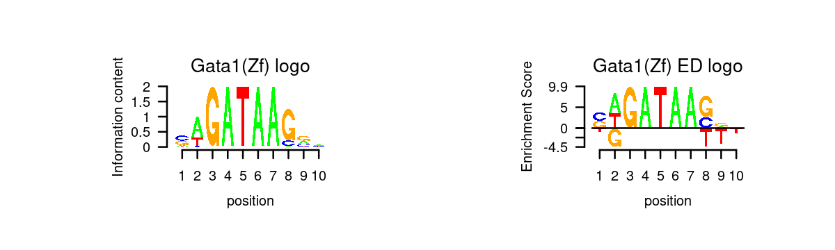
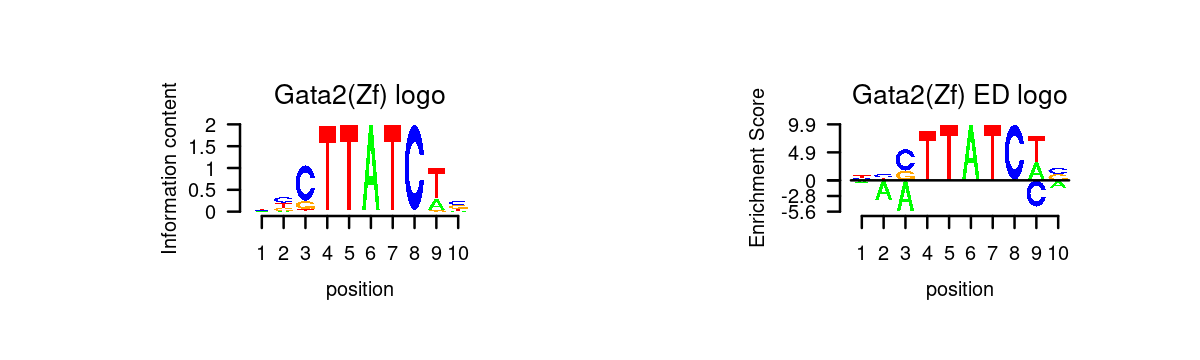
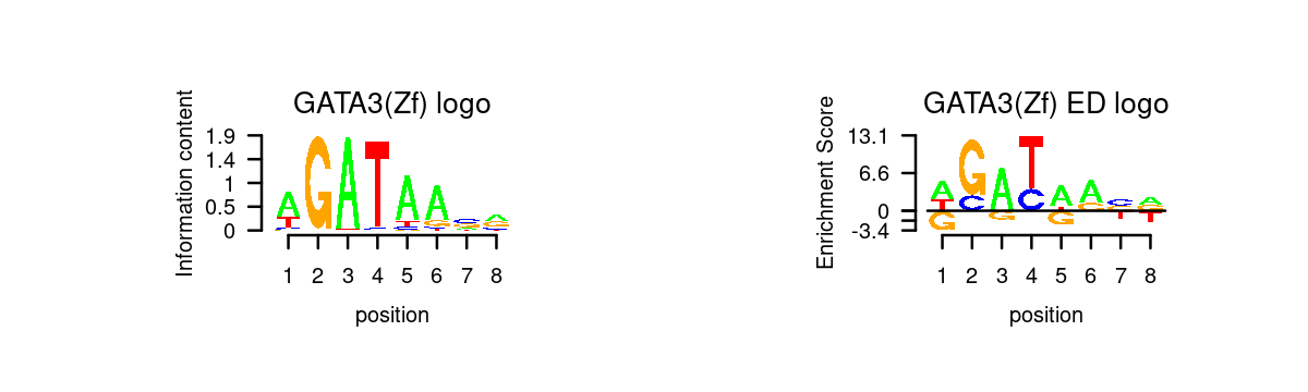
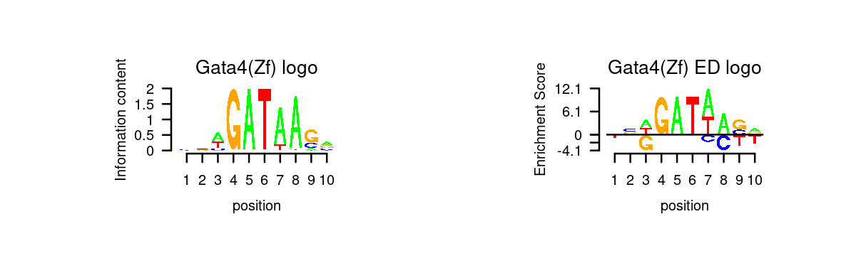
# 10 RUNX1(Runt) 27.712331 5.37659767 0.15396168GATA family
motif_names <- motif_res$motifs$motif
gene_names <- genescore_res$genes$SYMBOL
TF_motifs <- sort(unique(grep("^GATA\\d*$", motif_names, ignore.case=T, value=T)))
TF_genes <- sort(unique(grep("^GATA\\d*$", gene_names, ignore.case=T, value=T)))
common_genes <- intersect(toupper(TF_motifs), toupper(TF_genes))

motif_gene_table <- data.frame(motif = TF_motifs[match(common_genes, toupper(TF_motifs))],
                                      gene = TF_genes[match(common_genes, toupper(TF_genes))])
print(motif_gene_table)
# motif gene
# 1 Gata1 GATA1
# 2 Gata2 GATA2
# 3 GATA3 GATA3
# 4 Gata4 GATA4
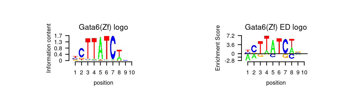
# 5 Gata6 GATA6# Plot GATA motifs in topic 4
k = 4
motif_order <- order(motif_res$mlog10P[,k], decreasing = T)
motifs <- rownames(motif_res$motifs[motif_order,])
motif_names <- motif_res$motifs[motif_order, "motif"]
selected_motifs <- unique(motifs[match(toupper(motif_gene_table$motif), toupper(motif_names))])
motif.dir <- paste0(homer.dir, "/homer_result_topic_", k, "/knownResults/")
for (i in 1:length(selected_motifs)){
plot_motif_logo(homer_res_topics, selected_motifs[i], k, motif.dir, type = "both")
}
| Version | Author | Date |
|---|---|---|
| 0fec792 | kevinlkx | 2021-02-01 |
| Version | Author | Date |
|---|---|---|
| 0fec792 | kevinlkx | 2021-02-01 |
| Version | Author | Date |
|---|---|---|
| 0fec792 | kevinlkx | 2021-02-01 |
| Version | Author | Date |
|---|---|---|
| 0fec792 | kevinlkx | 2021-02-01 |
| Version | Author | Date |
|---|---|---|
| 0fec792 | kevinlkx | 2021-02-01 |
- Plot motif enrichment (-log10 p-value) and gene scores
plots <- create_motif_gene_scatterplot(motif_res, genescore_res,
                                       motif_gene_table,
                                       k = 4,
                                       y = "-log10(p-value)",
                                       colors = colors_topics,
                                       max.overlaps = 10)

do.call(plot_grid,plots)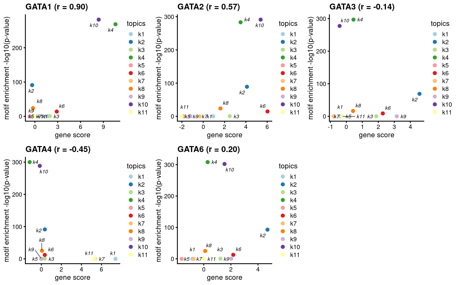
| Version | Author | Date |
|---|---|---|
| 0fec792 | kevinlkx | 2021-02-01 |
- Plot motif enrichment (zscore) and gene scores
plots <- create_motif_gene_scatterplot(motif_res, genescore_res,
                                       motif_gene_table,
                                       k = 4,
                                       y = "z-score",
                                       colors = colors_topics,
                                       max.overlaps = 10)

do.call(plot_grid,plots)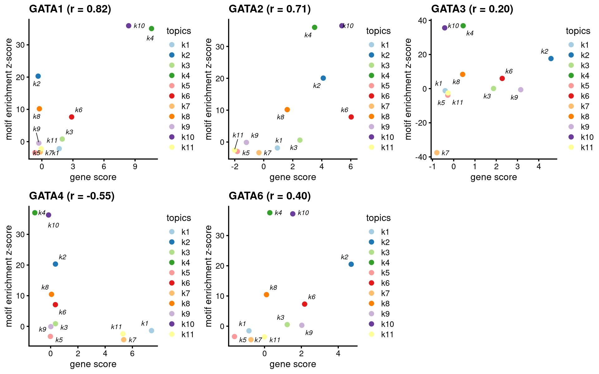
| Version | Author | Date |
|---|---|---|
| 0fec792 | kevinlkx | 2021-02-01 |
CEBP family
motif_names <- motif_res$motifs$motif
gene_names <- genescore_res$genes$SYMBOL
TF_motifs <- sort(unique(grep("^CEBP.?$", motif_names, ignore.case=T, value=T)))
TF_genes <- sort(unique(grep("^CEBP.?$", gene_names, ignore.case=T, value=T)))
motif_gene_table <- unique(data.frame(motif = c("CEBP"), gene = TF_genes))
print(motif_gene_table)
# motif gene
# 1 CEBP CEBPA
# 2 CEBP CEBPB
# 3 CEBP CEBPD
# 4 CEBP CEBPE
# 5 CEBP CEBPG
# 6 CEBP CEBPZ# Plot GATA motifs in topic 4
k = 1
motif_order <- order(motif_res$mlog10P[,k], decreasing = T)
motifs <- rownames(motif_res$motifs[motif_order,])
motif_names <- motif_res$motifs[motif_order, "motif"]
selected_motifs <- unique(motifs[match(toupper(motif_gene_table$motif), toupper(motif_names))])
motif.dir <- paste0(homer.dir, "/homer_result_topic_", k, "/knownResults/")
for (i in 1:length(selected_motifs)){
plot_motif_logo(homer_res_topics, selected_motifs[i], k, motif.dir, type = "both")
}
| Version | Author | Date |
|---|---|---|
| 0fec792 | kevinlkx | 2021-02-01 |
- Plot motif enrichment (-log10 p-value) and gene scores
plots <- create_motif_gene_scatterplot(motif_res, genescore_res,
                                       motif_gene_table,
                                       k = 1,
                                       y = "-log10(p-value)",
                                       colors = colors_topics,
                                       max.overlaps = 10)

do.call(plot_grid,plots)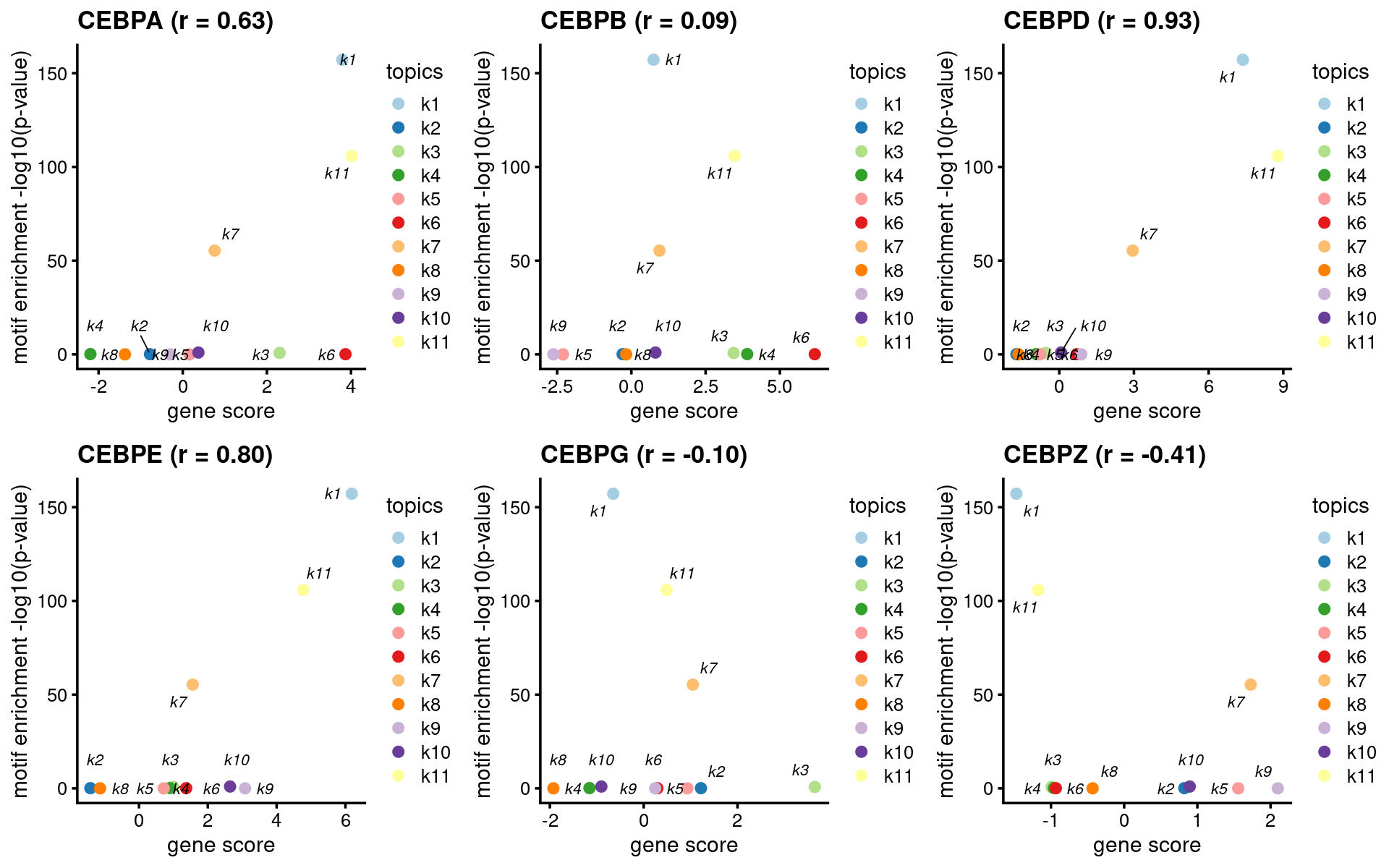
| Version | Author | Date |
|---|---|---|
| 0fec792 | kevinlkx | 2021-02-01 |
- Plot motif enrichment (zscore) and gene scores
plots <- create_motif_gene_scatterplot(motif_res, genescore_res,
                                       motif_gene_table,
                                       k = 1,
                                       y = "z-score",
                                       colors = colors_topics,
                                       max.overlaps = 10)

do.call(plot_grid,plots)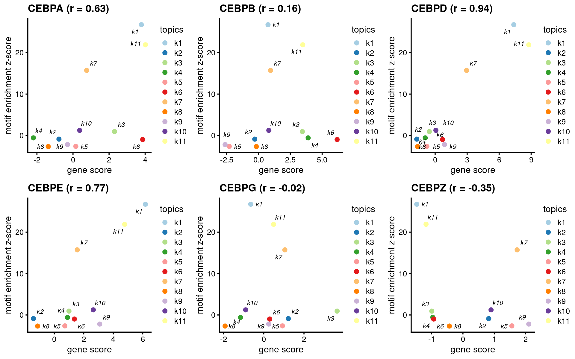
| Version | Author | Date |
|---|---|---|
| 0fec792 | kevinlkx | 2021-02-01 |
sessionInfo()# R version 3.6.1 (2019-07-05)
# Platform: x86_64-pc-linux-gnu (64-bit)
# Running under: Scientific Linux 7.4 (Nitrogen)
#
# Matrix products: default
# BLAS/LAPACK: /software/openblas-0.2.19-el7-x86_64/lib/libopenblas_haswellp-r0.2.19.so
#
# locale:
# [1] LC_CTYPE=en_US.UTF-8 LC_NUMERIC=C
# [3] LC_TIME=en_US.UTF-8 LC_COLLATE=en_US.UTF-8
# [5] LC_MONETARY=en_US.UTF-8 LC_MESSAGES=en_US.UTF-8
# [7] LC_PAPER=en_US.UTF-8 LC_NAME=C
# [9] LC_ADDRESS=C LC_TELEPHONE=C
# [11] LC_MEASUREMENT=en_US.UTF-8 LC_IDENTIFICATION=C
#
# attached base packages:
# [1] grid stats graphics grDevices utils datasets methods
# [8] base
#
# other attached packages:
# [1] Logolas_1.3.1 reshape2_1.4.3 DT_0.16 htmlwidgets_1.5.3
# [5] plotly_4.9.3 cowplot_1.1.1 ggrepel_0.9.1 ggplot2_3.3.3
# [9] tidyr_1.1.2 dplyr_1.0.3 fastTopics_0.4-29 Matrix_1.2-18
# [13] workflowr_1.6.2
#
# loaded via a namespace (and not attached):
# [1] nlme_3.1-140 mcmc_0.9-7 matrixStats_0.58.0 fs_1.3.1
# [5] bit64_4.0.5 progress_1.2.2 httr_1.4.2 rprojroot_2.0.2
# [9] tools_3.6.1 R6_2.5.0 irlba_2.3.3 DBI_1.1.0
# [13] lazyeval_0.2.2 colorspace_2.0-0 ade4_1.7-16 withr_2.4.1
# [17] tidyselect_1.1.0 prettyunits_1.1.1 bit_4.0.4 compiler_3.6.1
# [21] git2r_0.27.1 quantreg_5.83 SparseM_1.78 labeling_0.4.2
# [25] scales_1.1.1 SQUAREM_2021.1 quadprog_1.5-8 mixsqp_0.3-43
# [29] stringr_1.4.0 digest_0.6.27 rmarkdown_2.6 MCMCpack_1.5-0
# [33] pkgconfig_2.0.3 htmltools_0.5.1.1 invgamma_1.1 rlang_0.4.10
# [37] farver_2.0.3 generics_0.1.0 jsonlite_1.7.2 crosstalk_1.1.1
# [41] magrittr_2.0.1 Rcpp_1.0.6 munsell_0.5.0 ape_5.4-1
# [45] lifecycle_0.2.0 CVXR_1.0-9 stringi_1.5.3 whisker_0.4
# [49] yaml_2.2.1 MASS_7.3-53 Rtsne_0.15 plyr_1.8.6
# [53] parallel_3.6.1 promises_1.1.1 crayon_1.4.0 lattice_0.20-41
# [57] hms_1.0.0 knitr_1.30 pillar_1.4.7 seqinr_4.2-5
# [61] glue_1.4.2 evaluate_0.14 data.table_1.13.6 RcppParallel_5.0.2
# [65] vctrs_0.3.6 httpuv_1.5.4 MatrixModels_0.4-1 gtable_0.3.0
# [69] purrr_0.3.4 ashr_2.2-47 xfun_0.19 gridBase_0.4-7
# [73] Rmpfr_0.8-2 coda_0.19-4 later_1.1.0.1 viridisLite_0.3.0
# [77] truncnorm_1.0-8 tibble_3.0.6 conquer_1.0.2 gmp_0.6-2
# [81] ellipsis_0.3.1