Process data for Buenrostro 2018 scATAC-seq dataset
Kaixuan Luo
Last updated: 2020-11-10
Checks: 7 0
Knit directory: scATACseq-topics/
This reproducible R Markdown analysis was created with workflowr (version 1.6.2). The Checks tab describes the reproducibility checks that were applied when the results were created. The Past versions tab lists the development history.
Great! Since the R Markdown file has been committed to the Git repository, you know the exact version of the code that produced these results.
Great job! The global environment was empty. Objects defined in the global environment can affect the analysis in your R Markdown file in unknown ways. For reproduciblity it’s best to always run the code in an empty environment.
The command set.seed(20200729) was run prior to running the code in the R Markdown file. Setting a seed ensures that any results that rely on randomness, e.g. subsampling or permutations, are reproducible.
Great job! Recording the operating system, R version, and package versions is critical for reproducibility.
Nice! There were no cached chunks for this analysis, so you can be confident that you successfully produced the results during this run.
Great job! Using relative paths to the files within your workflowr project makes it easier to run your code on other machines.
Great! You are using Git for version control. Tracking code development and connecting the code version to the results is critical for reproducibility.
The results in this page were generated with repository version 614814b. See the Past versions tab to see a history of the changes made to the R Markdown and HTML files.
Note that you need to be careful to ensure that all relevant files for the analysis have been committed to Git prior to generating the results (you can use wflow_publish or wflow_git_commit). workflowr only checks the R Markdown file, but you know if there are other scripts or data files that it depends on. Below is the status of the Git repository when the results were generated:
Ignored files:
    Ignored:    .Rhistory
    Ignored:    .Rproj.user/

Untracked files:
    Untracked:  analysis/clusters_pca_structure_Cusanovich2018.Rmd
    Untracked:  analysis/process_data_Buenrostro2018_Chen2019.Rmd
    Untracked:  buenrostro2018.RData
    Untracked:  scripts/read_hema_counts.R

Unstaged changes:
    Modified:   analysis/plots_Lareau2019_bonemarrow.Rmd
    Modified:   scripts/fit_all_models_Buenrostro_2018.sbatch
Note that any generated files, e.g. HTML, png, CSS, etc., are not included in this status report because it is ok for generated content to have uncommitted changes.
These are the previous versions of the repository in which changes were made to the R Markdown (analysis/process_data_Buenrostro2018.Rmd) and HTML (docs/process_data_Buenrostro2018.html) files. If you’ve configured a remote Git repository (see ?wflow_git_remote), click on the hyperlinks in the table below to view the files as they were in that past version.
| File | Version | Author | Date | Message |
|---|---|---|---|---|
| Rmd | 614814b | kevinlkx | 2020-11-10 | process Buenrostro2018 data using Downloaded scATAC-seq processed data from GEO |
| Rmd | c113844 | kevinlkx | 2020-11-10 | wflow_rename(“analysis/process_data_Buenrostro2018.Rmd”, “analysis/process_data_Buenrostro2018_Chen2019pipeline.Rmd”) |
| html | c113844 | kevinlkx | 2020-11-10 | wflow_rename(“analysis/process_data_Buenrostro2018.Rmd”, “analysis/process_data_Buenrostro2018_Chen2019pipeline.Rmd”) |
| html | 1905c58 | kevinlkx | 2020-11-05 | Build site. |
| Rmd | 1da32f8 | kevinlkx | 2020-11-05 | set binarized counts as sparse matrix |
| html | 89b45be | kevinlkx | 2020-11-04 | Build site. |
| Rmd | 857e1e8 | kevinlkx | 2020-11-04 | process data from Buenrostro 2018 paper |
| html | 907fa65 | kevinlkx | 2020-11-04 | Build site. |
| Rmd | 12bf4b3 | kevinlkx | 2020-11-04 | process data from Buenrostro 2018 paper |
About Buenrostro 2018 dataset
Reference: Buenrostro, J. D. et al. Integrated Single-Cell Analysis Maps the Continuous Regulatory Landscape of Human Hematopoietic Differentiation. Cell 173, 1535–1548.e16 (2018).
Data were downloaded from GEO: GSE96772
RCC directory: /project2/mstephens/kevinluo/scATACseq-topics/data/Buenrostro_2018/
Processed data
Downloaded scATAC-seq processed data from GEO: GSE96769
GSE96769_PeakFile_20160207.bed.gzGSE96769_scATACseq_counts.txt.gz
Prepare data for topic modeling
library(Matrix)
library(tools)
library(readr)
library(data.table)
Load the fragment counts as a 2,953 x 491,437 sparse matrix.
# The first row has the sample names
file_counts <- "/project2/mstephens/kevinluo/scATACseq-topics/data/Buenrostro_2018/GEO_data/GSE96769_scATACseq_counts.txt.gz"
sample_names <- readLines(file_counts,n = 1)
sample_names <- unlist(strsplit(sample_names,"\t",fixed = TRUE))
sample_names <- unlist(strsplit(sample_names,";",fixed = TRUE))
sample_names <- sample_names[-1]

# Load the fragment counts as sparse matrix.
dat <- fread(file_counts,sep = "\t",skip = 1)
class(dat) <- "data.frame"
names(dat) <- c("i","j","x")
counts <- sparseMatrix(i = dat$i,j = dat$j,x = dat$x)
counts <- t(counts)
rownames(counts) <- sample_names
dim(counts)
[1] 2953 491437peaks
peaks <- fread("/project2/mstephens/kevinluo/scATACseq-topics/data/Buenrostro_2018/GEO_data/GSE96769_PeakFile_20160207.bed.gz")
peak_names <- paste(peaks$V1,peaks$V2,peaks$V3,sep = "_")
rownames(peaks) <- peak_names
cat(sprintf("Number of peaks: %d\n",nrow(peaks)))
Number of peaks: 491437colnames(counts) <- peak_namesPlot the distribution of fragment counts.
y <- table(summary(counts)$x)
x <- names(y)
y <- as.numeric(y)
plot(x,y,pch = 20,log = "y",cex = 0.65,
     xlab = "number of fragments mapping to peak",
     ylab = "number of peaks")
lines(x,y)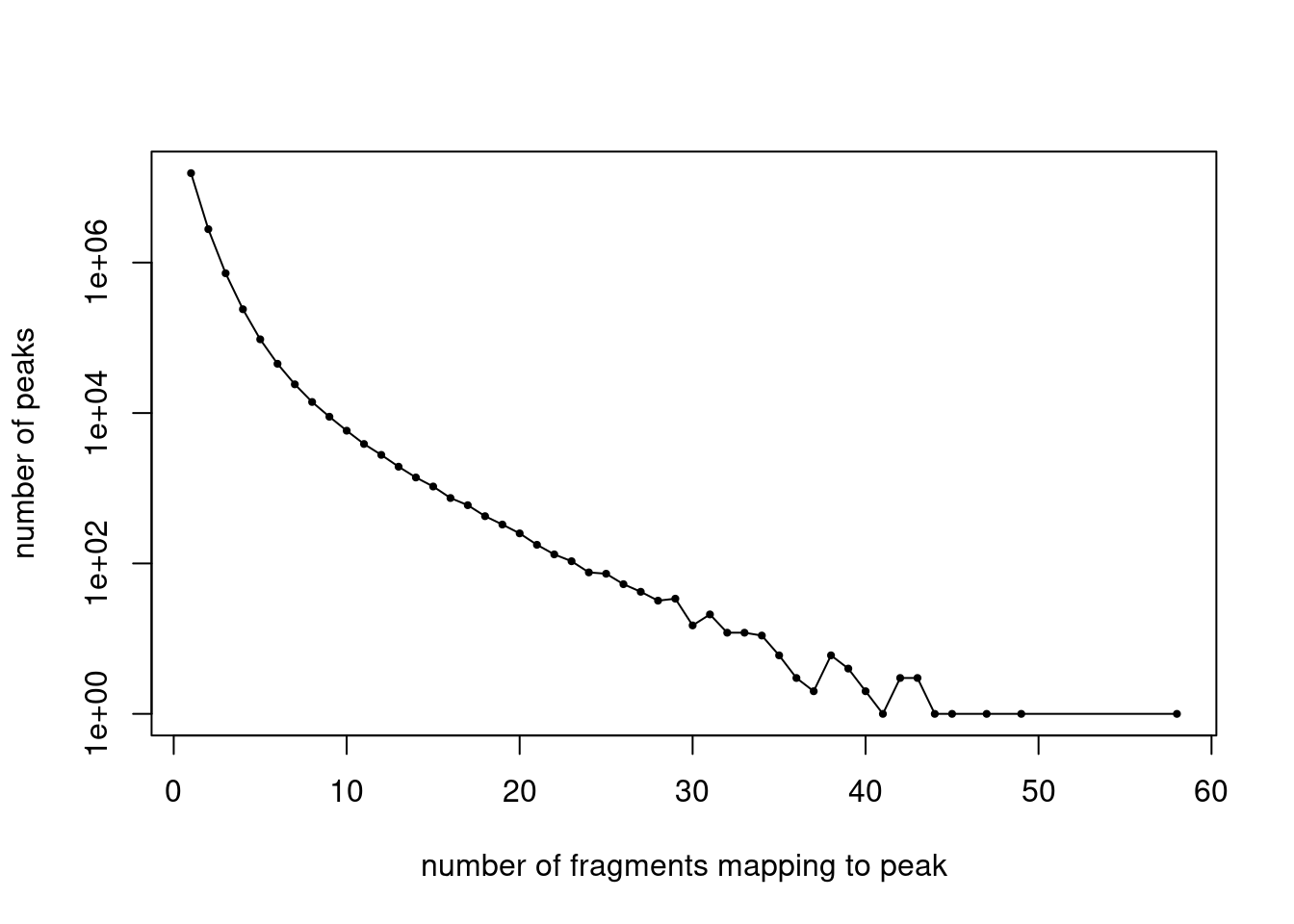
The supplementary Table S1 provides more details about these samples. https://ars.els-cdn.com/content/image/1-s2.0-S009286741830446X-mmc1.xlsx
Use the metadata.tsv from Chen et al. Genome Biology 2019 paper https://github.com/pinellolab/scATAC-benchmarking/tree/master/Real_Data/Buenrostro_2018/input/metadata.tsv)
samples_filtered <- read.table('/project2/mstephens/kevinluo/scATACseq-topics/data/Buenrostro_2018/data/input_Chen_2019/metadata.tsv', header = TRUE, stringsAsFactors=FALSE, quote="",row.names=1)
samples_filtered$name <- rownames(samples_filtered)

idx_samples_filtered <- match(samples_filtered$name, sample_names)
sample_names_filtered <- sample_names[idx_samples_filtered]
counts <- counts[idx_samples_filtered,]
samples <- samples_filtered[,c("name", "label")]
dim(counts)
[1] 2034 491437Remove peaks not exist in any of the cells
j <- which(colSums(counts > 0) >= 1)
peaks <- peaks[j,]
counts <- counts[,j]
cat(length(j), "peaks after filtering.  \n")
465536 peaks after filtering. Plot the distribution of filtered fragment counts.
y <- table(summary(counts)$x)
x <- names(y)
y <- as.numeric(y)
plot(x,y,pch = 20,log = "y",cex = 0.65,
     xlab = "number of fragments mapping to peak",
     ylab = "number of peaks")
lines(x,y)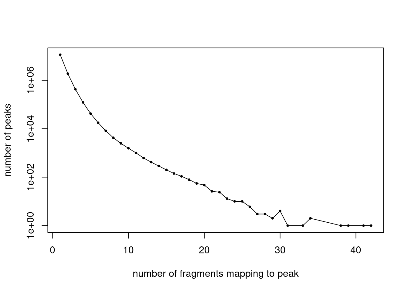
Binarize counts
binarized_counts <- as.matrix((counts > 0) + 0)
binarized_counts <- Matrix(binarized_counts, sparse = TRUE)

dim(binarized_counts)
[1] 2034 465536data.dir <- "/project2/mstephens/kevinluo/scATACseq-topics/data/Buenrostro_2018/processed_data/"
dir.create(data.dir, showWarnings = FALSE, recursive = TRUE)
saveRDS(counts, file.path(data.dir, "counts_Buenrostro_2018.rds"))
saveRDS(binarized_counts, file.path(data.dir, "binarized_counts_Buenrostro_2018.rds"))
save(list = c("samples", "peaks", "counts"),
file = file.path(data.dir, "Buenrostro_2018.RData"))
counts <- binarized_counts
save(list = c("samples", "peaks", "counts"),
file = file.path(data.dir, "Buenrostro_2018_binarized.RData"))data.dir <- "/project2/mstephens/kevinluo/scATACseq-topics/data/Buenrostro_2018/processed_data/"
load(file.path(data.dir, "Buenrostro_2018.RData"))
cat(sprintf("Loaded %d x %d counts matrix.\n",nrow(counts),ncol(counts)))Loaded 2034 x 465536 counts matrix.cat(sprintf("Number of samples (cells): %d\n",nrow(counts)))Number of samples (cells): 2034cat(sprintf("Number of peaks: %d\n",ncol(counts)))Number of peaks: 465536cat(sprintf("Proportion of counts that are non-zero: %0.1f%%.\n",
100*mean(counts > 0)))Proportion of counts that are non-zero: 1.5%.
sessionInfo()R version 3.6.1 (2019-07-05)
Platform: x86_64-pc-linux-gnu (64-bit)
Running under: Scientific Linux 7.4 (Nitrogen)
Matrix products: default
BLAS/LAPACK: /software/openblas-0.2.19-el7-x86_64/lib/libopenblas_haswellp-r0.2.19.so
locale:
[1] LC_CTYPE=en_US.UTF-8 LC_NUMERIC=C
[3] LC_TIME=en_US.UTF-8 LC_COLLATE=en_US.UTF-8
[5] LC_MONETARY=en_US.UTF-8 LC_MESSAGES=en_US.UTF-8
[7] LC_PAPER=en_US.UTF-8 LC_NAME=C
[9] LC_ADDRESS=C LC_TELEPHONE=C
[11] LC_MEASUREMENT=en_US.UTF-8 LC_IDENTIFICATION=C
attached base packages:
[1] tools stats graphics grDevices utils datasets methods
[8] base
other attached packages:
[1] data.table_1.12.8 readr_1.3.1 Matrix_1.2-18 workflowr_1.6.2
loaded via a namespace (and not attached):
[1] Rcpp_1.0.5 knitr_1.28 whisker_0.4 magrittr_1.5
[5] hms_0.5.3 lattice_0.20-38 R6_2.5.0 rlang_0.4.8
[9] stringr_1.4.0 grid_3.6.1 xfun_0.14 R.oo_1.23.0
[13] git2r_0.27.1 ellipsis_0.3.1 htmltools_0.4.0 yaml_2.2.0
[17] digest_0.6.27 rprojroot_1.3-2 lifecycle_0.2.0 tibble_3.0.4
[21] crayon_1.3.4 later_1.0.0 R.utils_2.9.2 vctrs_0.3.4
[25] promises_1.1.0 fs_1.3.1 glue_1.4.2 evaluate_0.14
[29] rmarkdown_2.1 stringi_1.4.6 pillar_1.4.6 compiler_3.6.1
[33] R.methodsS3_1.7.1 backports_1.1.10 httpuv_1.5.3.1 pkgconfig_2.0.3