cisTopic analysis for Buenrostro et al (2018) scATAC-seq data based on chromVAR processed counts with scPeaks (> 1 sample)
Kaixuan Luo
Last updated: 2020-11-27
Checks: 7 0
Knit directory: scATACseq-topics/
This reproducible R Markdown analysis was created with workflowr (version 1.6.2). The Checks tab describes the reproducibility checks that were applied when the results were created. The Past versions tab lists the development history.
Great! Since the R Markdown file has been committed to the Git repository, you know the exact version of the code that produced these results.
Great job! The global environment was empty. Objects defined in the global environment can affect the analysis in your R Markdown file in unknown ways. For reproduciblity it's best to always run the code in an empty environment.
The command set.seed(20200729) was run prior to running the code in the R Markdown file. Setting a seed ensures that any results that rely on randomness, e.g. subsampling or permutations, are reproducible.
Great job! Recording the operating system, R version, and package versions is critical for reproducibility.
Nice! There were no cached chunks for this analysis, so you can be confident that you successfully produced the results during this run.
Great job! Using relative paths to the files within your workflowr project makes it easier to run your code on other machines.
Great! You are using Git for version control. Tracking code development and connecting the code version to the results is critical for reproducibility.
The results in this page were generated with repository version 6acf4be. See the Past versions tab to see a history of the changes made to the R Markdown and HTML files.
Note that you need to be careful to ensure that all relevant files for the analysis have been committed to Git prior to generating the results (you can use wflow_publish or wflow_git_commit). workflowr only checks the R Markdown file, but you know if there are other scripts or data files that it depends on. Below is the status of the Git repository when the results were generated:
Ignored files:
    Ignored:    .Rhistory
    Ignored:    .Rproj.user/

Untracked files:
    Untracked:  analysis/clusters_pca_structure_Cusanovich2018.Rmd
    Untracked:  analysis/motif_analysis_Buenrostro2018_chomVAR_scPeaks.Rmd
    Untracked:  analysis/process_data_Buenrostro2018_Chen2019.Rmd
    Untracked:  buenrostro2018.RData
    Untracked:  scripts/fit_all_models_Buenrostro_2018_chromVar_scPeaks_filtered.sbatch

Unstaged changes:
    Modified:   analysis/plots_Lareau2019_bonemarrow.Rmd
    Modified:   analysis/process_data_Buenrostro2018.Rmd
    Modified:   code/motif_analysis.R
    Modified:   code/plots.R
    Modified:   scripts/fit_all_models_Buenrostro_2018.sbatch
Note that any generated files, e.g. HTML, png, CSS, etc., are not included in this status report because it is ok for generated content to have uncommitted changes.
These are the previous versions of the repository in which changes were made to the R Markdown (analysis/cisTopic_Buenrostro2018_chomVAR_scPeaks.Rmd) and HTML (docs/cisTopic_Buenrostro2018_chomVAR_scPeaks.html) files. If you've configured a remote Git repository (see ?wflow_git_remote), click on the hyperlinks in the table below to view the files as they were in that past version.
| File | Version | Author | Date | Message |
|---|---|---|---|---|
| Rmd | 6acf4be | kevinlkx | 2020-11-27 | run cisTopic analysis on Buenrostro2018_chomVAR_scPeaks dataset |
| html | 4e49f75 | kevinlkx | 2020-11-27 | Build site. |
| Rmd | 57e6ba9 | kevinlkx | 2020-11-27 | run cisTopic analysis on Buenrostro2018_chomVAR_scPeaks dataset |
Here we perform topic modeling analysis in the Buenrostro et al (2018) scATAC-seq data based on chromVAR processed counts with scPeaks (> 1 sample).
Load packages and functions
suppressWarnings(library(cisTopic))
source("code/motif_analysis.R")
Fit cisTopic models (using WarpLDA method)
Initializing the cisTopic object
- Load the binarized count matrix. In cisTopic, the rownames of these matrix must contain the region coordinates in position format (e.g. chr1:123456-134567)
data.dir <- "/project2/mstephens/kevinluo/scATACseq-topics/data/Buenrostro_2018/processed_data_Chen2019pipeline/chromVAR/"
load(file.path(data.dir, "Buenrostro_2018_binarized_scPeaks.RData"))
cat(sprintf("%d x %d counts matrix.\n",nrow(counts),ncol(counts)))
counts <- t(counts)
range(counts)
rownames(counts) <- paste0(peaks$chr, ":", peaks$start, "-",peaks$end)
cisTopicObject <- createcisTopicObject(counts, project.name='Buenrostro_2018_chromVAR_scPeaks')
dim(cisTopicObject@count.matrix)- Add metadata with the cell labels.
cisTopicObject <- addCellMetadata(cisTopicObject, cell.data = samples)- Fit cisTopic models (using WarpLDA). Fit 2 to 15 (by 1), and 20 to 50 (by 5) topics. See
scripts/fit_cisTopic_topics.R,scripts/fit_cisTopic_topics.sbatchandscripts/fit_cisTopic_Buenrostro_2018_chromVAR_scPeaks.shfor details.
cisTopicObject <- runWarpLDAModels(cisTopicObject, topic=c(2:15, 20, 25, 35, 40, 45, 50), seed=1, nCores=10, iterations = 1000, addModels=FALSE)Load cisTopic results
dir.out <- "/project2/mstephens/kevinluo/scATACseq-topics/output/cisTopic_Buenrostro_2018_chromVAR_scPeaks/binarized/"
cisTopicObject <- readRDS(paste0(dir.out, "/cisTopic-Buenrostro2018-binarized.rds"))
cat(sprintf("%d x %d counts matrix.\n",nrow(cisTopicObject@count.matrix),ncol(cisTopicObject@count.matrix)))
# 228965 x 2034 counts matrix.
Select cisTopic model
cisTopic (WarpLDA version) incorporates three different approaches (from left to right columns in the figure below) to select the best topic: From cisTopic tutorial website: - The log likelihood can be used to estimate the plausibility of a model parameter value, given the observed data (i.e. the highest the likelihood, the better the model). This is not recommended when running WarpLDA, as the curves stabilize rather than reaching a maximum.
The second derivative in each point of the likelihood curve, as it measures the changed in the curvature from point to point (i.e. the highest the second derivative means that the next model is not improving much more the log-likelihood) . This is not recommended when running CGS, as the curves tend to be noisier or reach a maximum. This is the default in this version of cisTopic.
The perplexity of each model (only for WarpLDA models) measures how well the model predicts the sample. The lower the perplexity is, the better the model.
par(mfrow=c(3,3))
cisTopicObject <- selectModel(cisTopicObject, type='maximum')
cisTopicObject <- selectModel(cisTopicObject, type='perplexity')
cisTopicObject <- selectModel(cisTopicObject, type='derivative')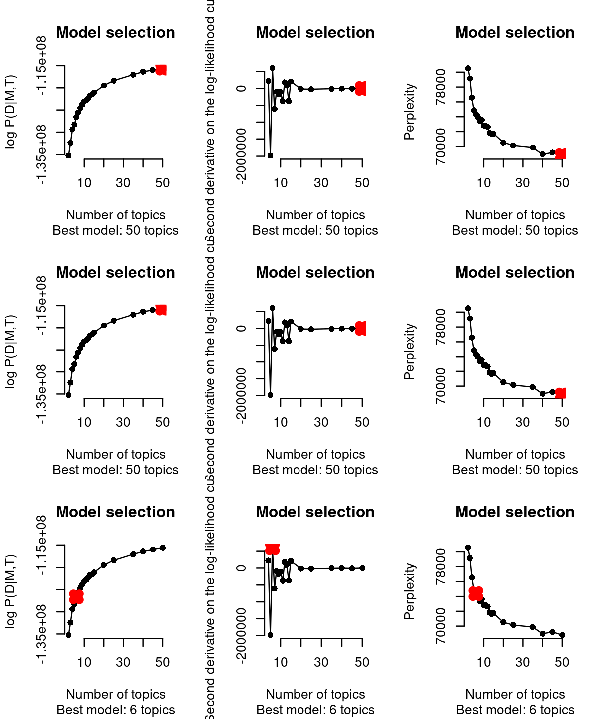
| Version | Author | Date |
|---|---|---|
| 4e49f75 | kevinlkx | 2020-11-27 |
# [1] "Are these CGS models? Please, use type=\"maximum\""Based on the second derivative (default in the WarpLDA version of cisTopic), we selected the cisTopic model with 6 topics. Alternatively, we can also manually select the number of topics with the parameter select.
Interpreting the cisTopic models
A. Identification of cell states using the cell-cisTopic distributions
The topic assignments to the cells (topic-cell matrix) are stored in cisTopicObject@selected.model$document_expects, with cells as columns, topics as rows. We can also retrieve the topic-cell and region-topic assignments using the function modelMatSelection.
fit.L <- t(cisTopicObject@selected.model$document_expects)
cellassign <- t(modelMatSelection(cisTopicObject, 'cell', 'Probability'))
all(cellassign == fit.L)
head(cellassign)
# [1] TRUE
#                                Topic1    Topic2    Topic3      Topic4
# BM1077-CLP-Frozen-160106-13 0.2452459 0.2616393 0.4275410 0.010491803
# BM1077-CLP-Frozen-160106-14 0.2354430 0.1932489 0.5181435 0.024472574
# BM1077-CLP-Frozen-160106-2  0.2482993 0.2100340 0.4957483 0.008503401
# BM1077-CLP-Frozen-160106-21 0.2216359 0.2357080 0.4028144 0.035180299
# BM1077-CLP-Frozen-160106-27 0.3217260 0.1294474 0.4224073 0.009084027
# BM1077-CLP-Frozen-160106-3  0.2869806 0.1351801 0.5252078 0.016066482
#                                  Topic5     Topic6
# BM1077-CLP-Frozen-160106-13 0.006557377 0.04852459
# BM1077-CLP-Frozen-160106-14 0.012658228 0.01603376
# BM1077-CLP-Frozen-160106-2  0.008503401 0.02891156
# BM1077-CLP-Frozen-160106-21 0.027264732 0.07739666
# BM1077-CLP-Frozen-160106-27 0.006056018 0.11127933
# BM1077-CLP-Frozen-160106-3  0.016066482 0.02049861
cisTopic includes wrapper functions to easily run Umap, tSNE, diffussion maps and PCA (the results are saved in the slot @dr$cell):
# run Umap of the cells
cisTopicObject <- runUmap(cisTopicObject, target='cell', seed=123, method='Probability')
# Loading required package: umap

# run tSNE of the cells
cisTopicObject <- runtSNE(cisTopicObject, target='cell', seed=123, pca=FALSE, method='Probability')
# Loading required package: Rtsne

summary(cisTopicObject@dr$cell)
#      Length Class  Mode
# Umap 4068   -none- numeric
# tSNE 4068   -none- numeric
cisTopic offers a unified visualization function (plotFeatures), which allows to visualize tSNE, diffussion maps, principal components and biplots (in 2/3D), colored by metadata and/or topic enrichment.
- Umap of the cells
par(mfrow=c(1,1))
plotFeatures(cisTopicObject, method='Umap', target='cell', topic_contr=NULL, colorBy='label',
             cex.legend = 0.8, factor.max=.75, dim=2, legend=TRUE,
             col.low='darkgreen', col.mid='yellow', col.high='brown1', intervals=10)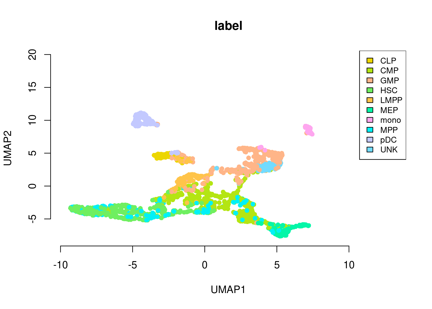
| Version | Author | Date |
|---|---|---|
| 4e49f75 | kevinlkx | 2020-11-27 |
Color the Umap by topic score (probability)
par(mfrow=c(2,3))

plotFeatures(cisTopicObject, method='Umap', target='cell', topic_contr='Probability',
             colorBy=NULL, cex.legend = 0.8, factor.max=.75, dim=2, legend=TRUE)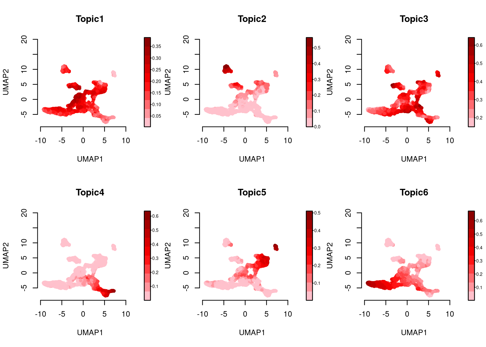
| Version | Author | Date |
|---|---|---|
| 4e49f75 | kevinlkx | 2020-11-27 |
- tSNE of the cells
par(mfrow=c(1,1))
plotFeatures(cisTopicObject, method='tSNE', target='cell', topic_contr=NULL, colorBy='label',
             cex.legend = 0.8, factor.max=.75, dim=2, legend=TRUE,
             col.low='darkgreen', col.mid='yellow', col.high='brown1', intervals=10)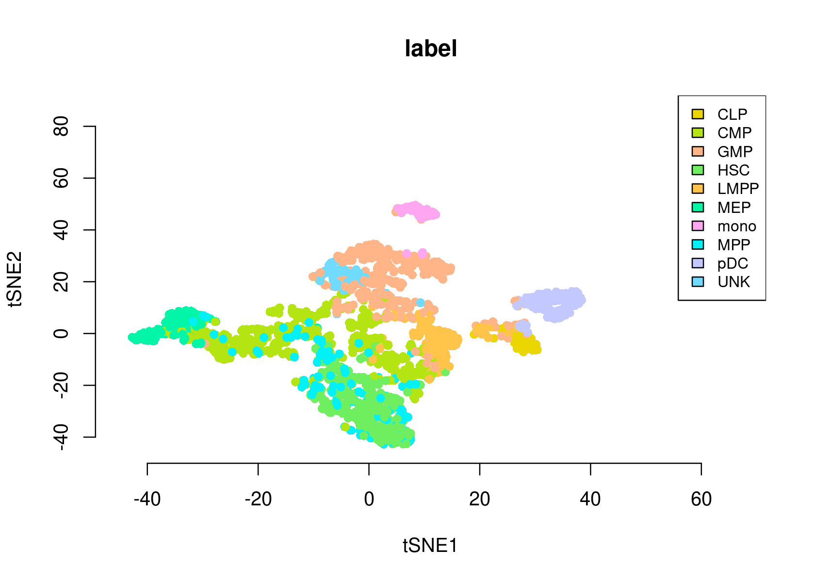
| Version | Author | Date |
|---|---|---|
| 4e49f75 | kevinlkx | 2020-11-27 |
Color the tSNE by topic score (probability)
par(mfrow=c(2,3))

plotFeatures(cisTopicObject, method='tSNE', target='cell', topic_contr='Probability',
             colorBy=NULL, cex.legend = 0.8, factor.max=.75, dim=2, legend=TRUE)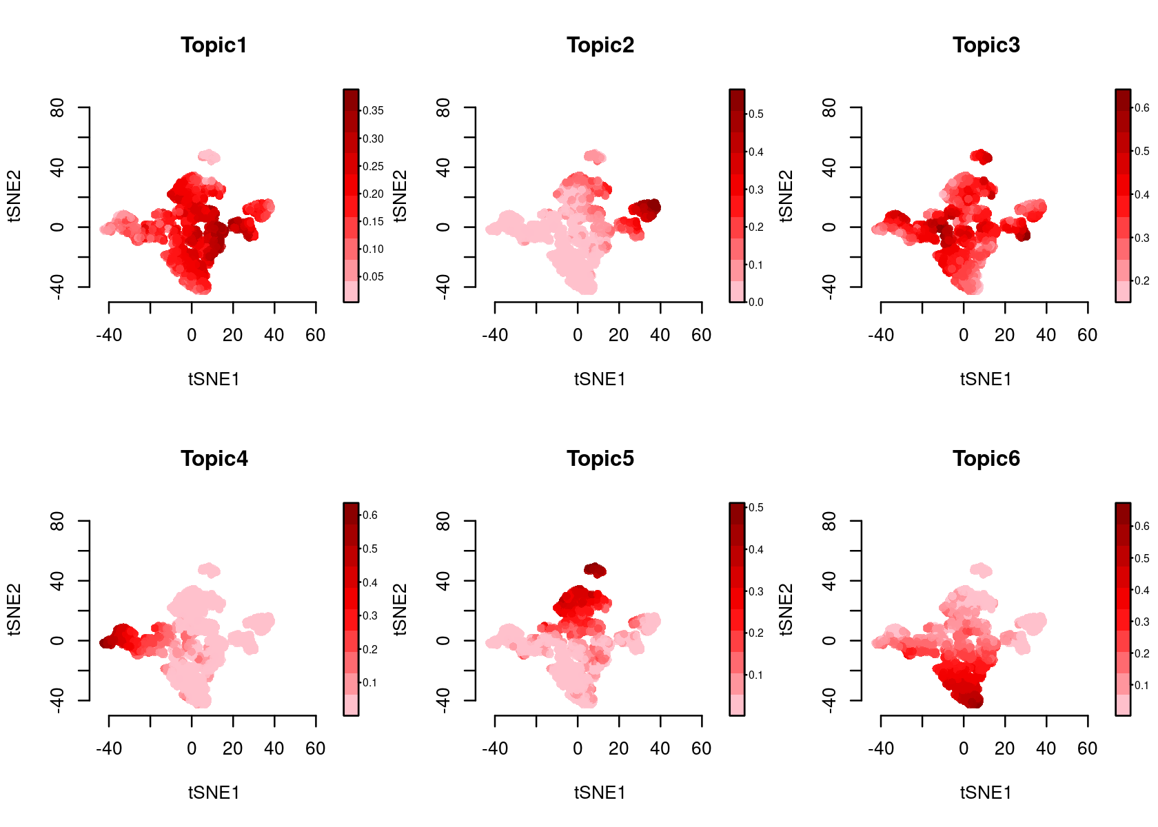
| Version | Author | Date |
|---|---|---|
| 4e49f75 | kevinlkx | 2020-11-27 |
- We can also generate a heatmap based on the cell-cisTopic distributions
cellTopicHeatmap(cisTopicObject, method='Probability', colorBy=c('label'))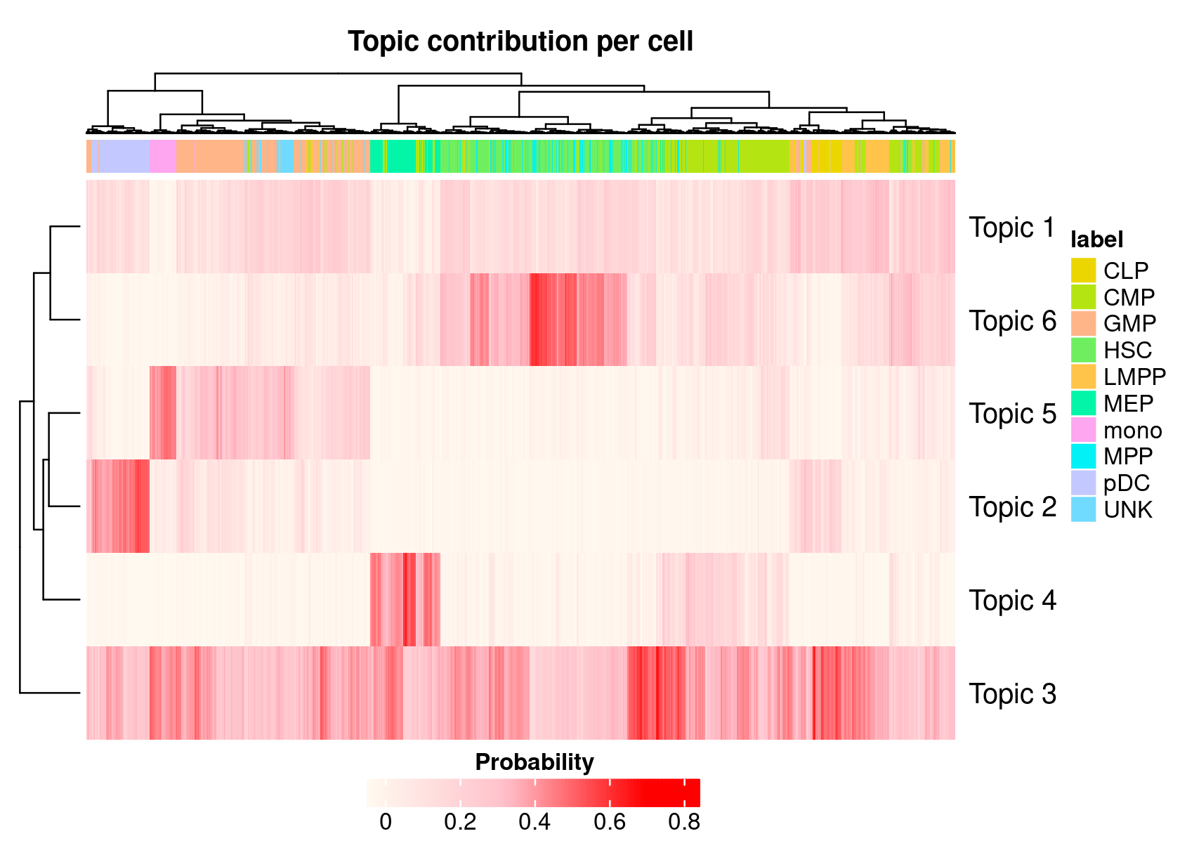
| Version | Author | Date |
|---|---|---|
| 4e49f75 | kevinlkx | 2020-11-27 |
cellTopicHeatmap(cisTopicObject, method='Z-score', colorBy=c('label'), col.low = "dodgerblue", col.mid = "floralwhite", col.high = "brown1")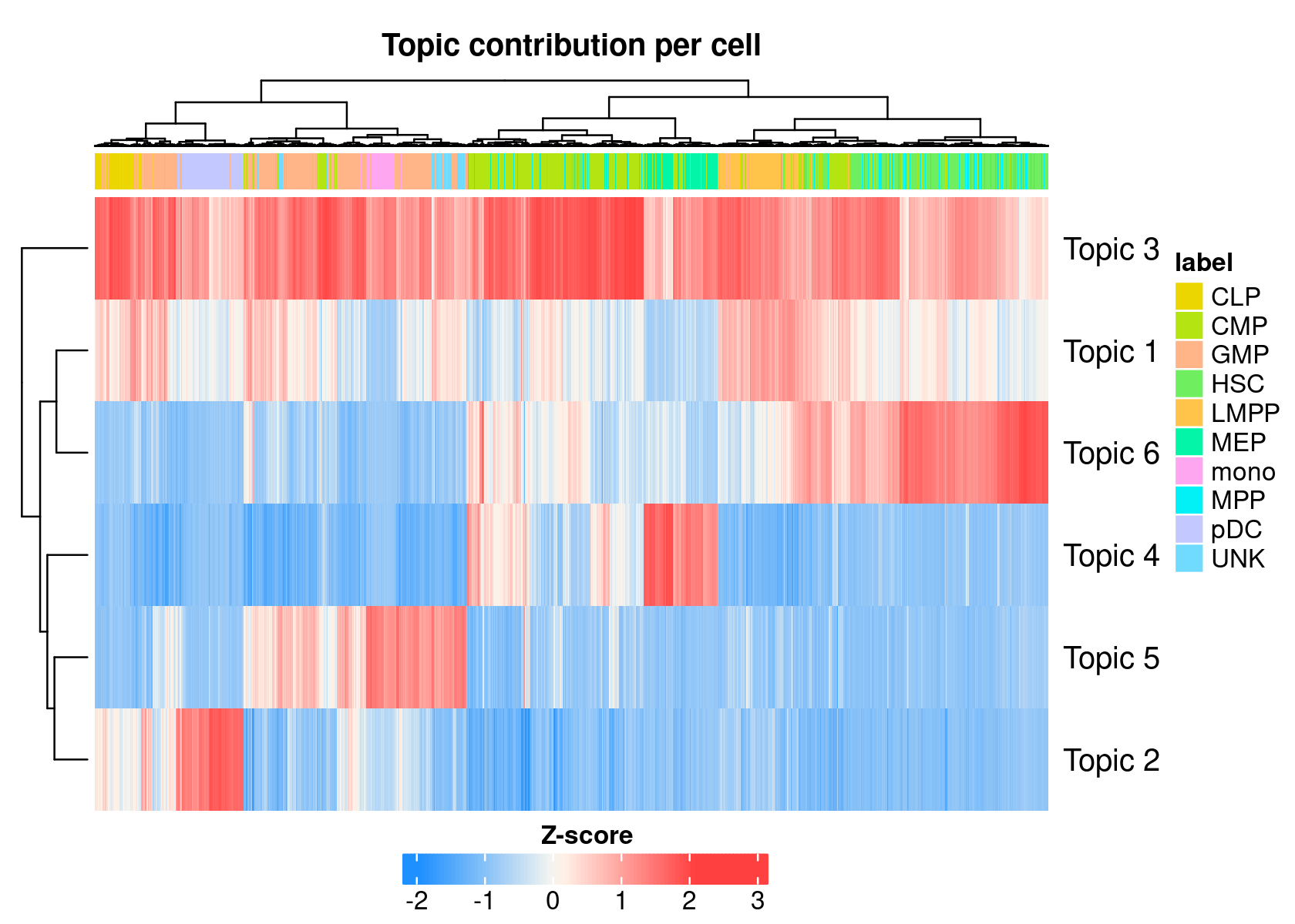
| Version | Author | Date |
|---|---|---|
| 4e49f75 | kevinlkx | 2020-11-27 |
Additionally, we can define clusters using the cell-topic matrix... [TO DO: add PCA plots and structure plots]
B. Analysis of the regulatory topics
Defining topics
To analyze the regions included in the cisTopics, the first step is always to derive a score that evaluates how likely is for a region to belong to a topic. getRegionsScores() calculates these scores based on the proportion of region specific assignments to a topic. These scores can be rescaled into the range [0,1], which will be useful for the binarization step (as it will force data to follow a gamma distribution shape). This information is stored in the region.data slot.
getRegionsScores gets region scores per topic using three different methods: Z-score, Probability, and NormTop. - 'Z-score' computes the Z-score for each topic assingment per cell/region. - 'Probability' divides the topic assignments by the total number of assignments in the cell/region in the last iteration plus alpha. - If using 'NormTop', regions are given an score defined by: \(β_{w, k} (\log β_{w,k} - 1 / K ∑_{k'} \log β_{w,k'})\).
- method = 'Z-score', scale = FALSE
cisTopicObject <- getRegionsScores(cisTopicObject, method='Z-score', scale=FALSE)
region.zscore <- cisTopicObject@region.data
print(head(region.zscore))
#                    seqnames  start    end width nCounts nCells Scores_Topic1
# chr1:10270-10769       chr1  10270  10769   499     230    230     0.7802464
# chr1:13253-13752       chr1  13253  13752   499      55     55    -0.5422576
# chr1:16000-16499       chr1  16000  16499   499      60     60     1.8549556
# chr1:96351-96850       chr1  96351  96850   499     107    107    -0.4175421
# chr1:115482-115981     chr1 115482 115981   499      32     32    -0.3118308
# chr1:237507-238006     chr1 237507 238006   499     111    111     1.8454276
#                    Scores_Topic2 Scores_Topic3 Scores_Topic4 Scores_Topic5
# chr1:10270-10769      -0.3356874    -1.0161348     0.1542347    1.46069380
# chr1:13253-13752      -0.5422576    -0.5422576    -0.5422576    0.22676227
# chr1:16000-16499      -0.5796736    -0.5796736     0.4637389   -0.57967362
# chr1:96351-96850      -0.4175421    -0.4175421    -0.4175421    2.04088334
# chr1:115482-115981    -0.4989292    -0.2182815     2.0269000   -0.49892923
# chr1:237507-238006    -0.7039260    -0.7039260     0.3234255   -0.05707508
#                    Scores_Topic6
# chr1:10270-10769      -1.0433527
# chr1:13253-13752       1.9422682
# chr1:16000-16499      -0.5796736
# chr1:96351-96850      -0.3707149
# chr1:115482-115981    -0.4989292
# chr1:237507-238006 -0.7039260- method = 'Z-score', scale = TRUE
cisTopicObject <- getRegionsScores(cisTopicObject, method='Z-score', scale=TRUE)
region.zscore <- cisTopicObject@region.data
print(head(region.zscore))
#                    seqnames  start    end width nCounts nCells Scores_Topic1
# chr1:10270-10769       chr1  10270  10769   499     230    230     0.6811759
# chr1:13253-13752       chr1  13253  13752   499      55     55     0.3468002
# chr1:16000-16499       chr1  16000  16499   499      60     60     0.9529004
# chr1:96351-96850       chr1  96351  96850   499     107    107     0.3783326
# chr1:115482-115981     chr1 115482 115981   499      32     32     0.4050602
# chr1:237507-238006     chr1 237507 238006   499     111    111     0.9504913
#                    Scores_Topic2 Scores_Topic3 Scores_Topic4 Scores_Topic5
# chr1:10270-10769       0.3932414     0.2216613     0.5198107     0.8488098
# chr1:13253-13752       0.3405103     0.3422997     0.3425733     0.5274608
# chr1:16000-16499       0.3309591     0.3327744     0.5985707     0.3174432
# chr1:96351-96850       0.3723464     0.3740494     0.3743099     0.9999067
# chr1:115482-115981     0.3515707     0.4247767     0.9963505     0.3384712
# chr1:237507-238006     0.2992412     0.3011426     0.5628649     0.4535419
#                    Scores_Topic6
# chr1:10270-10769       0.2197116
# chr1:13253-13752       0.9749634
# chr1:16000-16499       0.3370053
# chr1:96351-96850       0.3898641
# chr1:115482-115981     0.3574306
# chr1:237507-238006 0.3055740- method = 'Probability', scale = FALSE
cisTopicObject <- getRegionsScores(cisTopicObject, method='Probability', scale=FALSE)
region.probability <- cisTopicObject@region.data
print(head(region.probability))
#                    seqnames  start    end width nCounts nCells Scores_Topic1
# chr1:10270-10769       chr1  10270  10769   499     230    230  2.818780e-05
# chr1:13253-13752       chr1  13253  13752   499      55     55  4.200864e-08
# chr1:16000-16499       chr1  16000  16499   499      60     60  1.768564e-05
# chr1:96351-96850       chr1  96351  96850   499     107    107  4.200864e-08
# chr1:115482-115981     chr1 115482 115981   499      32     32  8.821815e-07
# chr1:237507-238006     chr1 237507 238006   499     111    111  2.818780e-05
#                    Scores_Topic2 Scores_Topic3 Scores_Topic4 Scores_Topic5
# chr1:10270-10769    2.324895e-05  2.563283e-07  3.995551e-05  6.214904e-05
# chr1:13253-13752    8.907642e-08  2.330257e-08  9.060207e-08  8.839874e-06
# chr1:16000-16499    8.907642e-08  2.330257e-08  1.639898e-05  6.747996e-08
# chr1:96351-96850    8.907642e-08  2.330257e-08  9.060207e-08  7.092144e-05
# chr1:115482-115981  8.907642e-08  7.223798e-07  2.455316e-05  6.747996e-08
# chr1:237507-238006  8.907642e-08  2.330257e-08  2.455316e-05  1.153907e-05
#                    Scores_Topic6
# chr1:10270-10769    5.073988e-08
# chr1:13253-13752    2.136149e-05
# chr1:16000-16499    5.073988e-08
# chr1:96351-96850    1.065537e-06
# chr1:115482-115981  5.073988e-08
# chr1:237507-238006 5.073988e-08- method = 'Probability', scale = TRUE
cisTopicObject <- getRegionsScores(cisTopicObject, method='Probability', scale=TRUE)
region.probability <- cisTopicObject@region.data
print(head(region.probability))
#                    seqnames  start    end width nCounts nCells Scores_Topic1
# chr1:10270-10769       chr1  10270  10769   499     230    230   0.119642857
# chr1:13253-13752       chr1  13253  13752   499      55     55   0.000000000
# chr1:16000-16499       chr1  16000  16499   499      60     60   0.075000000
# chr1:96351-96850       chr1  96351  96850   499     107    107   0.000000000
# chr1:115482-115981     chr1 115482 115981   499      32     32   0.003571429
# chr1:237507-238006     chr1 237507 238006   499     111    111   0.119642857
#                    Scores_Topic2 Scores_Topic3 Scores_Topic4 Scores_Topic5
# chr1:10270-10769       0.1027668   0.000729927    0.19383260    0.28571429
# chr1:13253-13752       0.0000000   0.000000000    0.00000000    0.04037267
# chr1:16000-16499       0.0000000   0.000000000    0.07929515    0.00000000
# chr1:96351-96850       0.0000000   0.000000000    0.00000000    0.32608696
# chr1:115482-115981     0.0000000   0.002189781    0.11894273    0.00000000
# chr1:237507-238006     0.0000000   0.000000000    0.11894273    0.05279503
#                    Scores_Topic6
# chr1:10270-10769     0.000000000
# chr1:13253-13752     0.086419753
# chr1:16000-16499     0.000000000
# chr1:96351-96850     0.004115226
# chr1:115482-115981   0.000000000
# chr1:237507-238006 0.000000000- method = 'NormTop', scale = FALSE
cisTopicObject <- getRegionsScores(cisTopicObject, method='NormTop', scale=FALSE)
region.NormTop <- cisTopicObject@region.data
print(head(region.NormTop))
#                    seqnames  start    end width nCounts nCells Scores_Topic1
# chr1:10270-10769       chr1  10270  10769   499     230    230  8.911007e-06
# chr1:13253-13752       chr1  13253  13752   499      55     55  0.000000e+00
# chr1:16000-16499       chr1  16000  16499   499      60     60  1.227631e-05
# chr1:96351-96850       chr1  96351  96850   499     107    107  0.000000e+00
# chr1:115482-115981     chr1 115482 115981   499      32     32 -1.290886e-07
# chr1:237507-238006     chr1 237507 238006   499     111    111  2.228603e-05
#                    Scores_Topic2 Scores_Topic3 Scores_Topic4 Scores_Topic5
# chr1:10270-10769    4.273959e-06 -2.364444e-07  2.406384e-05  6.029550e-05
# chr1:13253-13752    0.000000e+00  0.000000e+00  0.000000e+00  3.023777e-06
# chr1:16000-16499    0.000000e+00  0.000000e+00  1.076603e-05  0.000000e+00
# chr1:96351-96850    0.000000e+00  0.000000e+00  0.000000e+00  1.249909e-04
# chr1:115482-115981  0.000000e+00 -1.164380e-07  2.544592e-05  0.000000e+00
# chr1:237507-238006  0.000000e+00  0.000000e+00  1.724757e-05  2.455172e-06
#                    Scores_Topic6
# chr1:10270-10769    0.000000e+00
# chr1:13253-13752    1.836160e-05
# chr1:16000-16499    0.000000e+00
# chr1:96351-96850   -2.763661e-07
# chr1:115482-115981  0.000000e+00
# chr1:237507-238006 0.000000e+00- method = 'NormTop', scale = TRUE
cisTopicObject <- getRegionsScores(cisTopicObject, method='NormTop', scale=TRUE)
region.NormTop <- cisTopicObject@region.data
print(head(region.NormTop))
#                    seqnames  start    end width nCounts nCells Scores_Topic1
# chr1:10270-10769       chr1  10270  10769   499     230    230    0.04012664
# chr1:13253-13752       chr1  13253  13752   499      55     55    0.02409664
# chr1:16000-16499       chr1  16000  16499   499      60     60    0.04618047
# chr1:96351-96850       chr1  96351  96850   499     107    107    0.02409664
# chr1:115482-115981     chr1 115482 115981   499      32     32    0.02386442
# chr1:237507-238006     chr1 237507 238006   499     111    111    0.06418694
#                    Scores_Topic2 Scores_Topic3 Scores_Topic4 Scores_Topic5
# chr1:10270-10769      0.03249664    0.01740609    0.07905513    0.13121317
# chr1:13253-13752      0.02494510    0.01769429    0.02483142    0.03132216
# chr1:16000-16499      0.02494510    0.01769429    0.04909081    0.02604821
# chr1:96351-96850      0.02494510    0.01769429    0.02483142    0.24405234
# chr1:115482-115981    0.02494510    0.01755237    0.08216941    0.02604821
# chr1:237507-238006    0.02494510    0.01769429    0.06369585    0.03033042
#                    Scores_Topic6
# chr1:10270-10769      0.03183595
# chr1:13253-13752      0.06227577
# chr1:16000-16499      0.03183595
# chr1:96351-96850      0.03137779
# chr1:115482-115981    0.03183595
# chr1:237507-238006    0.03183595
BigWig files for observing the scored regions in the genome can be generated. Note that information on the length of the chromosomes has to be provided. These files can be uploaded in IGV or UCSC for visualisation. This information can be easily found in the TxDb objects of the corresponding genomes, for example.
## human hg19 gene annotation
suppressMessages(library(TxDb.Hsapiens.UCSC.hg19.knownGene))
txdb <- TxDb.Hsapiens.UCSC.hg19.knownGene

getBigwigFiles(cisTopicObject, path=paste0(dir.out, '/cisTopics_regionscores_normTop_asBW'), seqlengths=seqlengths(txdb))
However, many tools are limited to work with sets of regions rather than rankings of regions. Keywords, or the most contributing regions in a topic, can be used as a representative set of regions of the topic. binarizecisTopics() allows to select the top regions based on two methods:
method = "Predefined": to select a predefined number of regions (determined by the
cutoffsargument)method = "GammaFit" (default): to automatically select a threshold based on a fit of the scores to a gamma distribution. This is recommended when using
method="NormTop" and scale=TRUEingetRegionScores(). Note that the probability threshold must be provided by the user and it must be taken after the density (based on the fitted gamma distribution) is stabilised (i.e. in the tail of the distribution). Selected regions per topic will be stored as a list inobject@binarized.cisTopics.Select the top 2000 regions per topic.
par(mfrow=c(2,3))
cisTopicObject <- binarizecisTopics(cisTopicObject, method="Predefined", cutoffs=2000, plot=FALSE)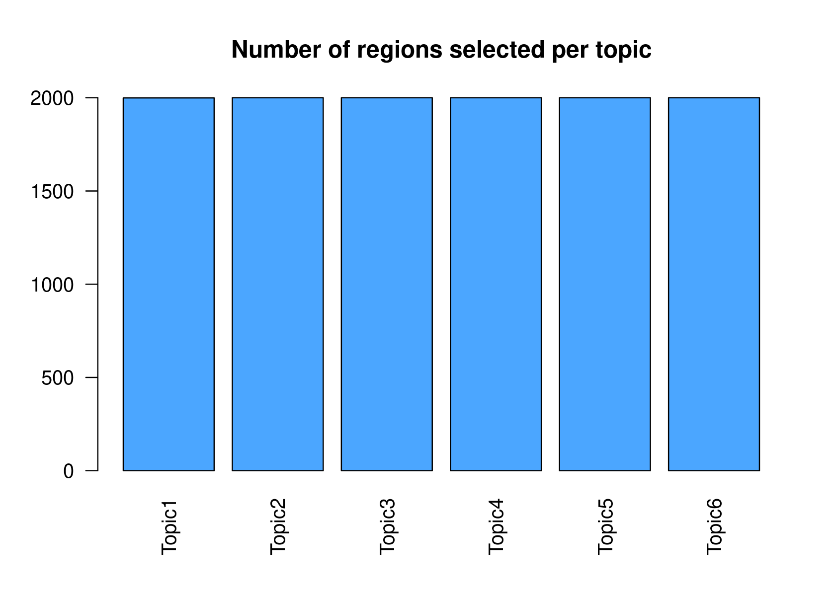
| Version | Author | Date |
|---|---|---|
| 4e49f75 | kevinlkx | 2020-11-27 |
summary(cisTopicObject@binarized.cisTopics)
#        Length Class      Mode
# Topic1 1      data.frame list
# Topic2 1      data.frame list
# Topic3 1      data.frame list
# Topic4 1      data.frame list
# Topic5 1      data.frame list
# Topic6 1 data.frame list- Select the regions based on the Gamma distributions fitted to the region scores.
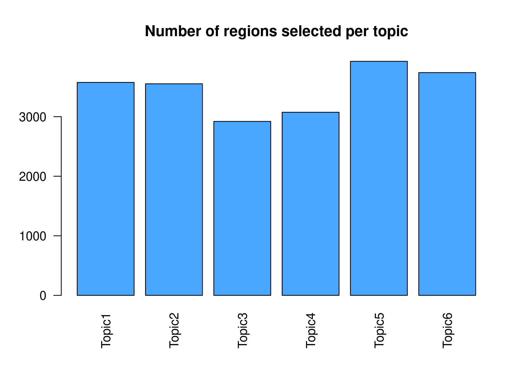
par(mfrow=c(2,3))
cisTopicObject <- binarizecisTopics(cisTopicObject, method="GammaFit", thrP=0.99, plot=TRUE)
# Loading required package: fitdistrplus
# Loading required package: MASS
#
# Attaching package: 'MASS'
# The following object is masked from 'package:plotly':
#
#     select
# Loading required package: survival
# Loading required package: npsurv
# Loading required package: lsei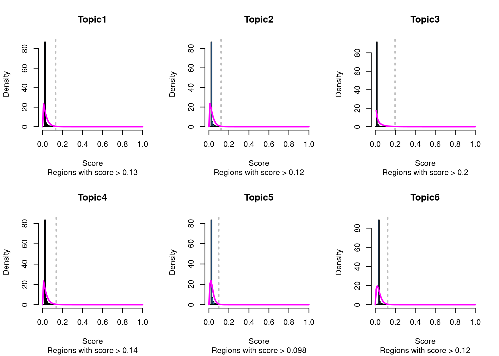
| Version | Author | Date |
|---|---|---|
| 4e49f75 | kevinlkx | 2020-11-27 |
| Version | Author | Date |
|---|---|---|
| 4e49f75 | kevinlkx | 2020-11-27 |
summary(cisTopicObject@binarized.cisTopics)
#        Length Class      Mode
# Topic1 1      data.frame list
# Topic2 1      data.frame list
# Topic3 1      data.frame list
# Topic4 1      data.frame list
# Topic5 1      data.frame list
# Topic6 1      data.frame list
The regions sets selected and distributions for each cisTopic can then be analized in different ways. They can also be exported to bed files to analyze with external tools:
getBedFiles(cisTopicObject, path=paste0(dir.out, '/cisTopics_selected_regions_asBED'))Topic visualization
Based on the topic scores for each region, different methods can be used for clustering and/or visualization.
cisTopic includes wrapper functions to easily run Umap, tSNE, diffussion maps and PCA (the results are saved in the slot @dr$region). In the case of regions, only high confidence regions (i.e. that pass the binarization threshold at least in 1 topic) are used:
cisTopicObject <- runtSNE(cisTopicObject, target='region', perplexity=200, check_duplicates=FALSE)
summary(cisTopicObject@dr$region)
#      Length Class  Mode
# tSNE 37378  -none- numeric
The function plotFeatures can also be used to visualize region-based tSNEs, diffussion maps, principal components and biplots (in 2/3D), colored by metadata and/or topic enrichment.
- tSNE plot of the regions
par(mfrow=c(1,1))
plotFeatures(cisTopicObject, method='tSNE', target='region', topic_contr=NULL, colorBy=c('nCells'), cex.legend = 0.8, factor.max=.75, dim=2, legend=TRUE, col.low='darkgreen', col.mid='yellow', col.high='brown1', intervals=10)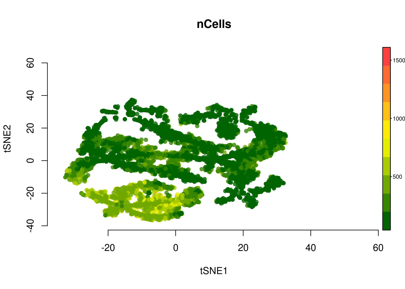
| Version | Author | Date |
|---|---|---|
| 4e49f75 | kevinlkx | 2020-11-27 |
Color the tSNE plot of the regions by topic scores (Z-score or probability)
# topic_contr: Color by topic distribution ('Z-score' or 'Probability').
par(mfrow=c(2,3))
plotFeatures(cisTopicObject, method='tSNE', target='region', topic_contr='Z-score', colorBy=NULL, cex.legend = 0.8, factor.max=.75, dim=2, legend=TRUE, col.low='darkgreen', col.mid='yellow', col.high='brown1')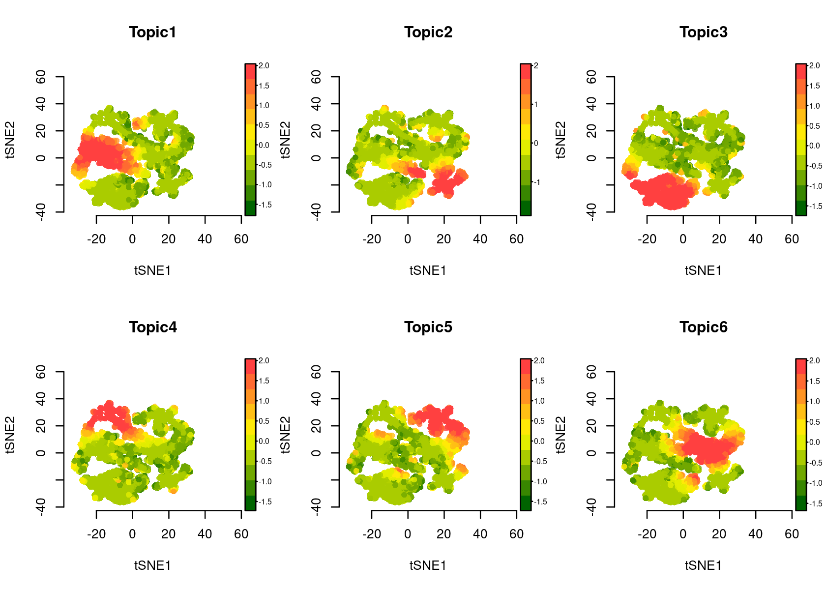
| Version | Author | Date |
|---|---|---|
| 4e49f75 | kevinlkx | 2020-11-27 |
plotFeatures(cisTopicObject, method='tSNE', target='region', topic_contr='Probability', colorBy=NULL, cex.legend = 0.8, factor.max=.75, dim=2, legend=TRUE)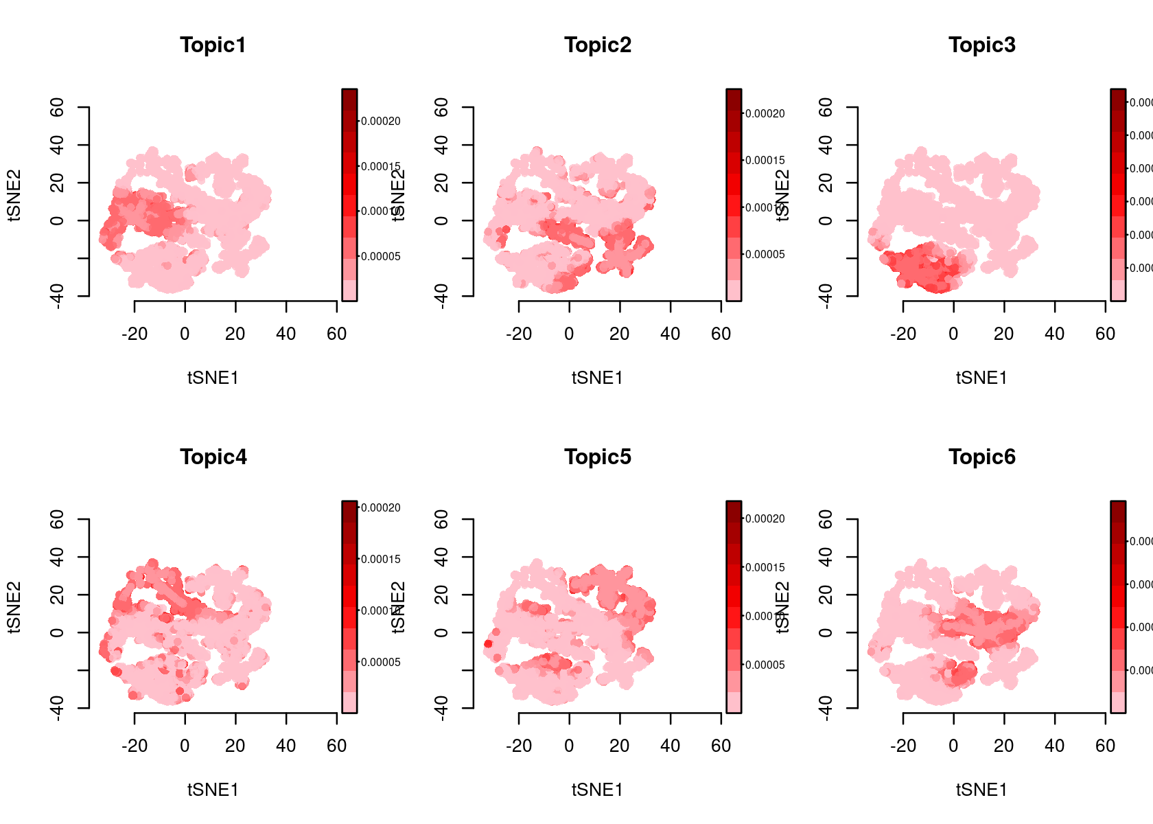
| Version | Author | Date |
|---|---|---|
| 4e49f75 | kevinlkx | 2020-11-27 |
Annotation to genes and GO terms
Another way of gaining insight on the topics is to link the regions to genes, and to determine GO terms (or pathways or any other type of gene-set) that are enriched within them.
cisTopic provides the function annotateRegions() to annotate regions to GO terms using the “TxDb” Bioconductor packages (replace ‘TxDb.Hsapiens.UCSC.hg19.knownGene’ by the appropiate organism package), and annotation databases (“OrgDb” packages).
suppressMessages(library(TxDb.Hsapiens.UCSC.hg19.knownGene))
suppressMessages(library(org.Hs.eg.db))
cisTopicObject <- annotateRegions(cisTopicObject, txdb=TxDb.Hsapiens.UCSC.hg19.knownGene, annoDb='org.Hs.eg.db')
# Loading required package: ChIPseeker
#
# Registered S3 method overwritten by 'enrichplot':
#   method               from
#   fortify.enrichResult DOSE
# ChIPseeker v1.20.0  For help: https://guangchuangyu.github.io/ChIPseeker
#
# If you use ChIPseeker in published research, please cite:
# Guangchuang Yu, Li-Gen Wang, Qing-Yu He. ChIPseeker: an R/Bioconductor package for ChIP peak annotation, comparison and visualization. Bioinformatics 2015, 31(14):2382-2383
# 'select()' returned 1:many mapping between keys and columns
# >> preparing features information...       2020-11-27 10:02:41 PM
# >> identifying nearest features...         2020-11-27 10:02:42 PM
# >> calculating distance from peak to TSS...    2020-11-27 10:02:47 PM
# >> assigning genomic annotation...         2020-11-27 10:02:47 PM
# >> adding gene annotation...           2020-11-27 10:03:03 PM
# >> assigning chromosome lengths            2020-11-27 10:03:03 PM
# >> done...                     2020-11-27 10:03:03 PM
We can use the region type annotations as region sets/signatures to check whether a topic is more enriched in a certain type of region.
par(mfrow=c(1,1))
signaturesHeatmap(cisTopicObject, selected.signatures = 'annotation')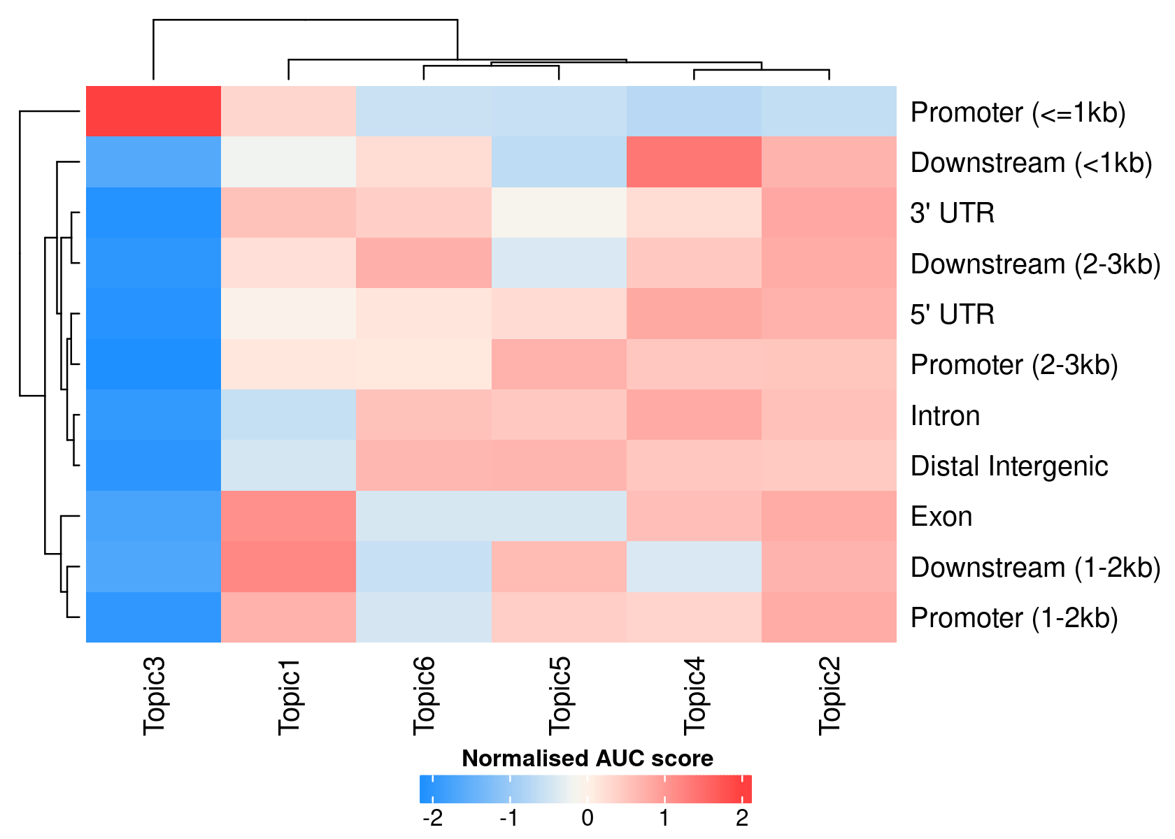
| Version | Author | Date |
|---|---|---|
| 4e49f75 | kevinlkx | 2020-11-27 |
plotFeatures(cisTopicObject, method='tSNE', target='region', topic_contr=NULL, colorBy=c('annotation'), cex.legend = 0.8, factor.max=.75, dim=2, legend=TRUE, intervals=20)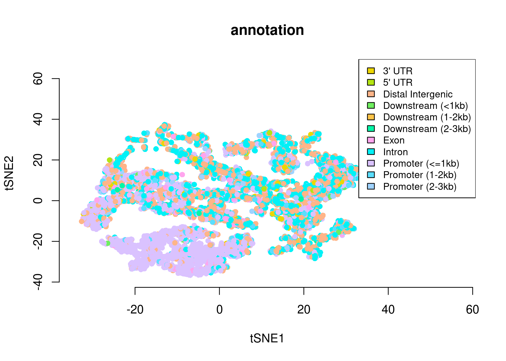
| Version | Author | Date |
|---|---|---|
| 4e49f75 | kevinlkx | 2020-11-27 |
Save cisTopicObject for further downstream analysis.
saveRDS(cisTopicObject, paste0(dir.out, "/cisTopic-Buenrostro2018-binarized-processed-1.rds"))GREAT GO annotation
For identifying enriched GO terms per topic, cisTopic provides a wrapper over rGREAT (Gu Z, 2017)[This analysis takes longer time]. The binarized topics (i.e. sets of top regions per topic) are used in this step. Results are stored in object@binarized.rGREAT.
cisTopicObject <- GREAT(cisTopicObject, genome='hg19', fold_enrichment=2, geneHits=1, sign=0.05, request_interval=10)We can visualize the enrichment results:
ontologyDotPlot(cisTopicObject, top=5, topics=c(6,10), var.y='name', order.by='Binom_Adjp_BH')Transcription factor motif enrichment
RcisTarget
It is also possible to identify enriched motifs within the topics and form cistromes (i.e. sets of sequences enriched for a given motif). To do this, we use RcisTarget (Aibar et al., 2017). RcisTarget tutorial
You can find the region-based database at: https://resources.aertslab.org/cistarget/ The list of all available databases is at https://resources.aertslab.org/cistarget/. Each database is stored in a .feather file.
Download the database (region based) to /project2/mstephens/kevinluo/cisTarget
dir.out <- "/project2/mstephens/kevinluo/scATACseq-topics/output/cisTopic_Buenrostro_2018_chromVAR_scPeaks/binarized/"
cisTopicObject <- readRDS(paste0(dir.out, "/cisTopic-Buenrostro2018-binarized-processed-1.rds"))
For this analysis, we first need to convert the cisTopic regions to the regions in the cisTarget databases (“ctx regions”).
We can do this in two ways:
- binarized, converting the binarized topic to a set of equivalent ctx regions (a region can map to more than one ctx region, and all regions which overlap more than the given threshold are taken). Results are stored in object@binarized.regions.to.Rct.
cisTopicObject <- binarizedcisTopicsToCtx(cisTopicObject, genome='hg19')
# Number of regions selected: 3181
# Number of regions selected: 3484
# Number of regions selected: 2607
# Number of regions selected: 3039
# Number of regions selected: 3894
# Number of regions selected: 3703
summary(cisTopicObject@binarized.regions.to.Rct)
head(cisTopicObject@binarized.regions.to.Rct[[1]])
#        Length Class  Mode
# Topic1 3181   -none- character
# Topic2 3484   -none- character
# Topic3 2607   -none- character
# Topic4 3039   -none- character
# Topic5 3894   -none- character
# Topic6 3703   -none- character
# [1] "chr1-reg212" "chr1-reg413" "chr1-reg422" "chr1-reg519" "chr1-reg534"
# [6] "chr1-reg607"- Based on the maximum overlap. This is useful if we need to use the scores (a region is mapped to its most overlapping ctx region). This information is stored in object@region.data.
cisTopicObject <- scoredRegionsToCtx(cisTopicObject, genome='hg19')
# Number of regions selected: 163147
dim(cisTopicObject@region.data)
print(cisTopicObject@region.data[1:3,])
# [1] 228965     25
#                  seqnames start   end width nCounts nCells Scores_Topic1
# chr1:10270-10769     chr1 10270 10769   500     230    230    0.04012664
# chr1:13253-13752     chr1 13253 13752   500      55     55    0.02409664
# chr1:16000-16499     chr1 16000 16499   500      60     60    0.04618047
#                  Scores_Topic2 Scores_Topic3 Scores_Topic4 Scores_Topic5
# chr1:10270-10769    0.03249664    0.01740609    0.07905513    0.13121317
# chr1:13253-13752    0.02494510    0.01769429    0.02483142    0.03132216
# chr1:16000-16499    0.02494510    0.01769429    0.04909081    0.02604821
#                  Scores_Topic6       annotation geneChr geneStart geneEnd
# chr1:10270-10769    0.03183595 Promoter (1-2kb)       1     11874   14409
# chr1:13253-13752    0.06227577 Promoter (1-2kb)       1     11874   14409
# chr1:16000-16499    0.03183595 Promoter (<=1kb)       1     14362   16765
#                  geneLength geneStrand    geneId transcriptId distanceToTSS
# chr1:10270-10769       2536          1 100287102   uc001aaa.3         -1105
# chr1:13253-13752       2536          1 100287102   uc010nxr.1          1379
# chr1:16000-16499       2404          2    653635   uc009vis.3           266
#                          ENSEMBL  SYMBOL
# chr1:10270-10769 ENSG00000223972 DDX11L1
# chr1:13253-13752 ENSG00000223972 DDX11L1
# chr1:16000-16499 ENSG00000227232  WASH7P
#                                                  GENENAME CtxLabels
# chr1:10270-10769            DEAD/H-box helicase 11 like 1 chr1-reg3
# chr1:13253-13752            DEAD/H-box helicase 11 like 1      <NA>
# chr1:16000-16499 WAS protein family homolog 7, pseudogene chr1-reg5
We can run RcisTarget in each topic using the wrapper function topicsRcisTarget(). This function uses the binarized topic regions converted to ctx regions.
pathToFeather <- "/project2/mstephens/kevinluo/cisTarget/hg19-regions-9species.all_regions.mc9nr.feather"
cisTopicObject <- topicsRcisTarget(cisTopicObject, genome='hg19', pathToFeather, reduced_database=FALSE, nesThreshold=3, rocthr=0.005, maxRank=20000, nCores=5)
HOMER
We can use HOMER to do TF motif enrichment for target regions (peaks)
homer.result <- vector("list", length(cisTopicObject@binarized.cisTopics))
for(i in 1:length(cisTopicObject@binarized.cisTopics)){
  target_regions <- read.table(sprintf('%s/cisTopics_selected_regions_asBED/Topic_%s.bed', dir.out, i), sep = "\t", header =  FALSE, stringsAsFactors = FALSE)
  target_regions[,4] <- paste0(target_regions[,1], ":",target_regions[,2], "-",target_regions[,3])
  file.regions <- sprintf('%s/cisTopics_selected_regions_asBED/Topic_%s_regions.bed', dir.out, i)
  write.table(target_regions, file.regions, col.names = FALSE, row.names = FALSE, quote = FALSE, sep = "\t")
  homer.result[[i]] <- homer_motif_enrichment('/project2/xinhe/software/homer/bin/findMotifsGenome.pl',
                                              file.regions,
                                              genome = 'hg19',
                                              result.dir = sprintf('%s/motif_enrichment_homer/Topic_%s/', dir.out, i),
                                              region.size = 200,
                                              n.cores = 5,
                                              run = FALSE)
}
#
# HOMER command:
# /project2/xinhe/software/homer/bin/findMotifsGenome.pl /project2/mstephens/kevinluo/scATACseq-topics/output/cisTopic_Buenrostro_2018_chromVAR_scPeaks/binarized//cisTopics_selected_regions_asBED/Topic_1_regions.bed hg19 /project2/mstephens/kevinluo/scATACseq-topics/output/cisTopic_Buenrostro_2018_chromVAR_scPeaks/binarized//motif_enrichment_homer/Topic_1/ -len 8,10,12 -size 200 -mis 2 -S 25 -p 5
#
# HOMER command:
# /project2/xinhe/software/homer/bin/findMotifsGenome.pl /project2/mstephens/kevinluo/scATACseq-topics/output/cisTopic_Buenrostro_2018_chromVAR_scPeaks/binarized//cisTopics_selected_regions_asBED/Topic_2_regions.bed hg19 /project2/mstephens/kevinluo/scATACseq-topics/output/cisTopic_Buenrostro_2018_chromVAR_scPeaks/binarized//motif_enrichment_homer/Topic_2/ -len 8,10,12 -size 200 -mis 2 -S 25 -p 5
#
# HOMER command:
# /project2/xinhe/software/homer/bin/findMotifsGenome.pl /project2/mstephens/kevinluo/scATACseq-topics/output/cisTopic_Buenrostro_2018_chromVAR_scPeaks/binarized//cisTopics_selected_regions_asBED/Topic_3_regions.bed hg19 /project2/mstephens/kevinluo/scATACseq-topics/output/cisTopic_Buenrostro_2018_chromVAR_scPeaks/binarized//motif_enrichment_homer/Topic_3/ -len 8,10,12 -size 200 -mis 2 -S 25 -p 5
#
# HOMER command:
# /project2/xinhe/software/homer/bin/findMotifsGenome.pl /project2/mstephens/kevinluo/scATACseq-topics/output/cisTopic_Buenrostro_2018_chromVAR_scPeaks/binarized//cisTopics_selected_regions_asBED/Topic_4_regions.bed hg19 /project2/mstephens/kevinluo/scATACseq-topics/output/cisTopic_Buenrostro_2018_chromVAR_scPeaks/binarized//motif_enrichment_homer/Topic_4/ -len 8,10,12 -size 200 -mis 2 -S 25 -p 5
#
# HOMER command:
# /project2/xinhe/software/homer/bin/findMotifsGenome.pl /project2/mstephens/kevinluo/scATACseq-topics/output/cisTopic_Buenrostro_2018_chromVAR_scPeaks/binarized//cisTopics_selected_regions_asBED/Topic_5_regions.bed hg19 /project2/mstephens/kevinluo/scATACseq-topics/output/cisTopic_Buenrostro_2018_chromVAR_scPeaks/binarized//motif_enrichment_homer/Topic_5/ -len 8,10,12 -size 200 -mis 2 -S 25 -p 5
#
# HOMER command:
# /project2/xinhe/software/homer/bin/findMotifsGenome.pl /project2/mstephens/kevinluo/scATACseq-topics/output/cisTopic_Buenrostro_2018_chromVAR_scPeaks/binarized//cisTopics_selected_regions_asBED/Topic_6_regions.bed hg19 /project2/mstephens/kevinluo/scATACseq-topics/output/cisTopic_Buenrostro_2018_chromVAR_scPeaks/binarized//motif_enrichment_homer/Topic_6/ -len 8,10,12 -size 200 -mis 2 -S 25 -p 5
sessionInfo()
# R version 3.6.1 (2019-07-05)
# Platform: x86_64-pc-linux-gnu (64-bit)
# Running under: Scientific Linux 7.4 (Nitrogen)
#
# Matrix products: default
# BLAS/LAPACK: /software/openblas-0.2.19-el7-x86_64/lib/libopenblas_haswellp-r0.2.19.so
#
# locale:
#  [1] LC_CTYPE=en_US.UTF-8       LC_NUMERIC=C
#  [3] LC_TIME=en_US.UTF-8        LC_COLLATE=en_US.UTF-8
#  [5] LC_MONETARY=en_US.UTF-8    LC_MESSAGES=en_US.UTF-8
#  [7] LC_PAPER=en_US.UTF-8       LC_NAME=C
#  [9] LC_ADDRESS=C               LC_TELEPHONE=C
# [11] LC_MEASUREMENT=en_US.UTF-8 LC_IDENTIFICATION=C
#
# attached base packages:
#  [1] stats4    parallel  grid      stats     graphics  grDevices utils
#  [8] datasets  methods   base
#
# other attached packages:
#  [1] doRNG_1.8.2
#  [2] rngtools_1.5
#  [3] foreach_1.5.1
#  [4] ChIPseeker_1.20.0
#  [5] org.Hs.eg.db_3.7.0
#  [6] TxDb.Hsapiens.UCSC.hg19.knownGene_3.2.2
#  [7] GenomicFeatures_1.36.3
#  [8] AnnotationDbi_1.46.0
#  [9] Biobase_2.42.0
# [10] GenomicRanges_1.36.0
# [11] GenomeInfoDb_1.20.0
# [12] IRanges_2.18.1
# [13] S4Vectors_0.22.1
# [14] BiocGenerics_0.30.0
# [15] fitdistrplus_1.0-14
# [16] npsurv_0.4-0
# [17] lsei_1.2-0
# [18] survival_2.44-1.1
# [19] MASS_7.3-53
# [20] ComplexHeatmap_1.20.0
# [21] fastcluster_1.1.25
# [22] scatterplot3d_0.3-41
# [23] plotly_4.9.0
# [24] ggplot2_3.3.2
# [25] Rtsne_0.15
# [26] umap_0.2.7.0
# [27] cisTopic_0.3.0
# [28] workflowr_1.6.2
#
# loaded via a namespace (and not attached):
#   [1] reticulate_1.16             R.utils_2.10.1
#   [3] tidyselect_1.1.0            RSQLite_2.1.1
#   [5] htmlwidgets_1.5.2           BiocParallel_1.18.0
#   [7] munsell_0.5.0               codetools_0.2-16
#   [9] withr_2.3.0                 RcisTarget_1.9.2
#  [11] colorspace_2.0-0            GOSemSim_2.10.0
#  [13] knitr_1.30                  DOSE_3.10.2
#  [15] git2r_0.27.1                urltools_1.7.3
#  [17] GenomeInfoDbData_1.2.1      polyclip_1.10-0
#  [19] bit64_0.9-7                 farver_2.0.3
#  [21] rprojroot_1.3-2             vctrs_0.3.5
#  [23] generics_0.0.2              lambda.r_1.2.3
#  [25] xfun_0.19                   doParallel_1.0.14
#  [27] R6_2.5.0                    bitops_1.0-6
#  [29] fgsea_1.15.1                gridGraphics_0.4-1
#  [31] DelayedArray_0.10.0         promises_1.1.1
#  [33] scales_1.1.1                ggraph_1.0.2
#  [35] enrichplot_1.4.0            gtable_0.3.0
#  [37] rlang_0.4.8                 GlobalOptions_0.1.2
#  [39] text2vec_0.5.1              splines_3.6.1
#  [41] rtracklayer_1.44.0          lazyeval_0.2.2
#  [43] europepmc_0.3               yaml_2.2.0
#  [45] reshape2_1.4.3              backports_1.2.0
#  [47] httpuv_1.5.4                qvalue_2.16.0
#  [49] tools_3.6.1                 feather_0.3.3
#  [51] gridBase_0.4-7              ggplotify_0.0.3
#  [53] ellipsis_0.3.1              gplots_3.0.1.1
#  [55] RColorBrewer_1.1-2          ggridges_0.5.1
#  [57] Rcpp_1.0.5                  plyr_1.8.6
#  [59] doMC_1.3.7                  progress_1.2.2
#  [61] zlibbioc_1.30.0             purrr_0.3.4
#  [63] RCurl_1.98-1.1              prettyunits_1.1.1
#  [65] openssl_1.4.3               GetoptLong_1.0.4
#  [67] viridis_0.5.1               cowplot_1.1.0
#  [69] SummarizedExperiment_1.14.1 ggrepel_0.8.2
#  [71] fs_1.3.1                    magrittr_1.5
#  [73] data.table_1.13.2           RSpectra_0.15-0
#  [75] futile.options_1.0.1        DO.db_2.9
#  [77] circlize_0.4.11             triebeard_0.3.0
#  [79] mlapi_0.1.0                 whisker_0.4
#  [81] matrixStats_0.57.0          hms_0.5.3
#  [83] mime_0.9                    evaluate_0.14
#  [85] xtable_1.8-4                XML_3.98-1.20
#  [87] AUCell_1.13.0               gridExtra_2.3
#  [89] shape_1.4.5                 compiler_3.6.1
#  [91] biomaRt_2.40.1              tibble_3.0.4
#  [93] KernSmooth_2.23-15          crayon_1.3.4
#  [95] R.oo_1.24.0                 htmltools_0.5.0
#  [97] later_1.1.0.1               snow_0.4-3
#  [99] tidyr_1.1.2                 RcppParallel_5.0.2
# [101] DBI_1.1.0                   tweenr_1.0.1
# [103] formatR_1.7                 boot_1.3-23
# [105] Matrix_1.2-18               gdata_2.18.0
# [107] R.methodsS3_1.8.1           igraph_1.2.4.1
# [109] pkgconfig_2.0.3             rvcheck_0.1.3
# [111] GenomicAlignments_1.20.1    xml2_1.3.2
# [113] annotate_1.62.0             lda_1.4.2
# [115] XVector_0.24.0              stringr_1.4.0
# [117] digest_0.6.27               graph_1.60.0
# [119] Biostrings_2.52.0           rmarkdown_2.5
# [121] fastmatch_1.1-0             GSEABase_1.44.0
# [123] shiny_1.5.0                 Rsamtools_2.0.0
# [125] gtools_3.8.1                rjson_0.2.20
# [127] lifecycle_0.2.0             jsonlite_1.6
# [129] futile.logger_1.4.3         viridisLite_0.3.0
# [131] askpass_1.1                 pillar_1.4.7
# [133] lattice_0.20-41             plotrix_3.7-6
# [135] fastmap_1.0.1               httr_1.4.2
# [137] GO.db_3.8.2                 glue_1.4.2
# [139] UpSetR_1.4.0                iterators_1.0.13
# [141] bit_1.1-14                  ggforce_0.2.2
# [143] stringi_1.5.3               blob_1.2.0
# [145] caTools_1.17.1.2            doSNOW_1.0.18
# [147] memoise_1.1.0               dplyr_1.0.2