Visualize and interpret topics in Cusanovich2018 data
Kaixuan Luo
Last updated: 2020-09-11
Checks: 7 0
Knit directory: scATACseq-topics/
This reproducible R Markdown analysis was created with workflowr (version 1.6.2). The Checks tab describes the reproducibility checks that were applied when the results were created. The Past versions tab lists the development history.
Great! Since the R Markdown file has been committed to the Git repository, you know the exact version of the code that produced these results.
Great job! The global environment was empty. Objects defined in the global environment can affect the analysis in your R Markdown file in unknown ways. For reproduciblity it’s best to always run the code in an empty environment.
The command set.seed(20200729) was run prior to running the code in the R Markdown file. Setting a seed ensures that any results that rely on randomness, e.g. subsampling or permutations, are reproducible.
Great job! Recording the operating system, R version, and package versions is critical for reproducibility.
Nice! There were no cached chunks for this analysis, so you can be confident that you successfully produced the results during this run.
Great job! Using relative paths to the files within your workflowr project makes it easier to run your code on other machines.
Great! You are using Git for version control. Tracking code development and connecting the code version to the results is critical for reproducibility.
The results in this page were generated with repository version 6d64de6. See the Past versions tab to see a history of the changes made to the R Markdown and HTML files.
Note that you need to be careful to ensure that all relevant files for the analysis have been committed to Git prior to generating the results (you can use wflow_publish or wflow_git_commit). workflowr only checks the R Markdown file, but you know if there are other scripts or data files that it depends on. Below is the status of the Git repository when the results were generated:
Ignored files:
    Ignored:    .Rhistory
    Ignored:    .Rproj.user/
Note that any generated files, e.g. HTML, png, CSS, etc., are not included in this status report because it is ok for generated content to have uncommitted changes.
These are the previous versions of the repository in which changes were made to the R Markdown (analysis/plots_Cusanovich2018.Rmd) and HTML (docs/plots_Cusanovich2018.html) files. If you’ve configured a remote Git repository (see ?wflow_git_remote), click on the hyperlinks in the table below to view the files as they were in that past version.
| File | Version | Author | Date | Message |
|---|---|---|---|---|
| Rmd | 6d64de6 | kevinlkx | 2020-09-11 | add t-SNE and membership pie charts |
| html | 7c0b14f | kevinlkx | 2020-09-11 | Build site. |
| Rmd | dc70e46 | kevinlkx | 2020-09-11 | add t-SNE and membership pie charts |
| html | 5a8479b | kevinlkx | 2020-09-10 | Build site. |
| Rmd | b9993e2 | kevinlkx | 2020-09-10 | initial structure plots |
Here we examine and compare the topic modeling results for the scATAC-seq dataset from the mouse single-cell atlas paper Cusanovich et al (2018)
Load the packages used in the analysis below, as well as additional functions that will be used to generate some of the plots.
library(tools)
library(dplyr)
library(fastTopics)
library(ggplot2)
library(cowplot)
library(mapplots)
source("code/plots.R")set.seed(1)Cusanovich 2018 mouse scATAC-seq dataset
Load the data and Poisson NMF model fit
Load the data
data.dir <- "/project2/mstephens/kevinluo/scATACseq-topics/data/Cusanovich_2018/processed_data/"
load(file.path(data.dir, "Cusanovich_2018.RData"))
cat(sprintf("%d x %d counts matrix.\n",nrow(counts),ncol(counts)))
rm(counts)
# 81173 x 436206 counts matrix.
About the samples: The study measured single cell chromatin accessibility for 17 samples spanning 13 different tissues in 8-week old mice.
cat(nrow(samples), "samples (cells). \n")
# 81173 samples (cells).
Tissues:
samples$tissue <- as.factor(samples$tissue)
cat(length(levels(samples$tissue)), "tissues. \n")
table(samples$tissue)
# 13 tissues.
#
#       BoneMarrow       Cerebellum            Heart           Kidney
#             8403             2278             7650             6431
#   LargeIntestine            Liver             Lung PreFrontalCortex
#             7086             6167             9996             5959
#   SmallIntestine           Spleen           Testes           Thymus
#             4077             4020             2723             7617
#       WholeBrain
#             8766
Cell types labels:
samples$cell_label <- as.factor(samples$cell_label)
cat(length(levels(samples$cell_label)), "cell types \n")
table(samples$cell_label)
# 40 cell types
#
#          Activated B cells       Alveolar macrophages
#                        500                        559
#                 Astrocytes                    B cells
#                       1666                       5772
#             Cardiomyocytes   Cerebellar granule cells
#                       4076                       4099
#            Collecting duct                 Collisions
#                        164                       1218
#                     DCT/CD            Dendritic cells
#                        506                        958
#   Distal convoluted tubule Endothelial I (glomerular)
#                        319                        552
#        Endothelial I cells       Endothelial II cells
#                        952                       3019
#                Enterocytes              Erythroblasts
#                       4783                       2811
#            Ex. neurons CPN          Ex. neurons CThPN
#                       1832                       1540
#           Ex. neurons SCPN  Hematopoietic progenitors
#                       1466                       3425
#                Hepatocytes           Immature B cells
#                       5664                        571
#         Inhibitory neurons              Loop of henle
#                       1828                        815
#                Macrophages                  Microglia
#                        711                        422
#                  Monocytes                   NK cells
#                       1173                        321
#           Oligodendrocytes                  Podocytes
#                       1558                        498
#            Proximal tubule         Proximal tubule S3
#                       2570                        594
#             Purkinje cells         Regulatory T cells
#                        320                        507
#          SOM+ Interneurons                      Sperm
#                        553                       2089
#                    T cells         Type I pneumocytes
#                       8954                       1622
#        Type II pneumocytes                    Unknown
#                        157                      10029
Load the results of running fit_poisson_nmf on the Cusanovich2018 data, with different algorithms, and for various choices of \(k\) (the number of “topics”).
out.dir <- "/project2/mstephens/kevinluo/scATACseq-topics/output/Cusanovich_2018"
load(file.path(out.dir, "/compiled.fits.Cusanovich2018.RData"))
Select all scd-ex model fits
fits <- fits[grep("scd-ex", names(fits))]Structure plots
The structure plots below summarize the topic proportions in the samples grouped by different tissues.
\(k = 2\):
fit_poisson_nmf <- fits[["fit-Cusanovich2018-scd-ex-k=2"]]

p.structure_plot <- structure_plot(poisson2multinom(fit_poisson_nmf),
                     grouping = samples[,"tissue"],
                     n = 2000,gap = 40,num_threads = 4,verbose = FALSE)
print(p.structure_plot)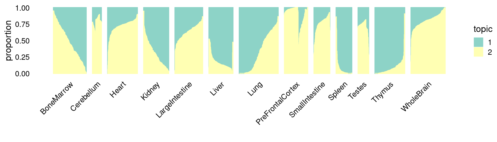
| Version | Author | Date |
|---|---|---|
| 5a8479b | kevinlkx | 2020-09-10 |
\(k = 3\):
fit_poisson_nmf <- fits[["fit-Cusanovich2018-scd-ex-k=3"]]

p.structure_plot <- structure_plot(poisson2multinom(fit_poisson_nmf),
                     grouping = samples[,"tissue"],
                     n = 2000,gap = 40,num_threads = 4,verbose = FALSE)
print(p.structure_plot)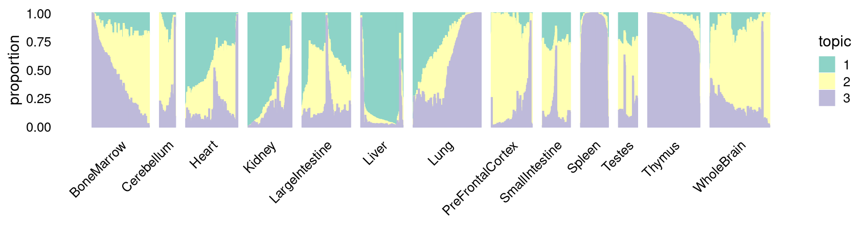
| Version | Author | Date |
|---|---|---|
| 5a8479b | kevinlkx | 2020-09-10 |
\(k = 4\):
fit_poisson_nmf <- fits[["fit-Cusanovich2018-scd-ex-k=4"]]

p.structure_plot <- structure_plot(poisson2multinom(fit_poisson_nmf),
                     grouping = samples[,"tissue"],
                     n = 2000,gap = 40,num_threads = 4,verbose = FALSE)
print(p.structure_plot)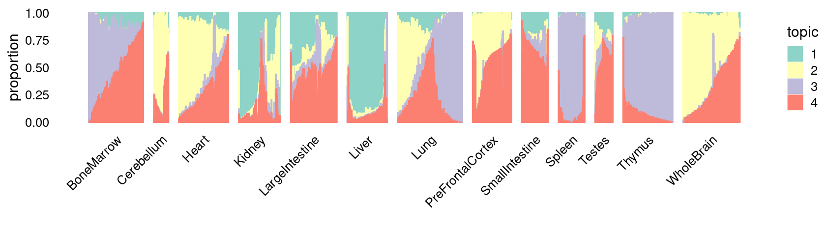
| Version | Author | Date |
|---|---|---|
| 5a8479b | kevinlkx | 2020-09-10 |
\(k = 5\):
fit_poisson_nmf <- fits[["fit-Cusanovich2018-scd-ex-k=5"]]

p.structure_plot <- structure_plot(poisson2multinom(fit_poisson_nmf),
                     grouping = samples[,"tissue"],
                     n = 2000,gap = 40,num_threads = 4,verbose = FALSE)
print(p.structure_plot)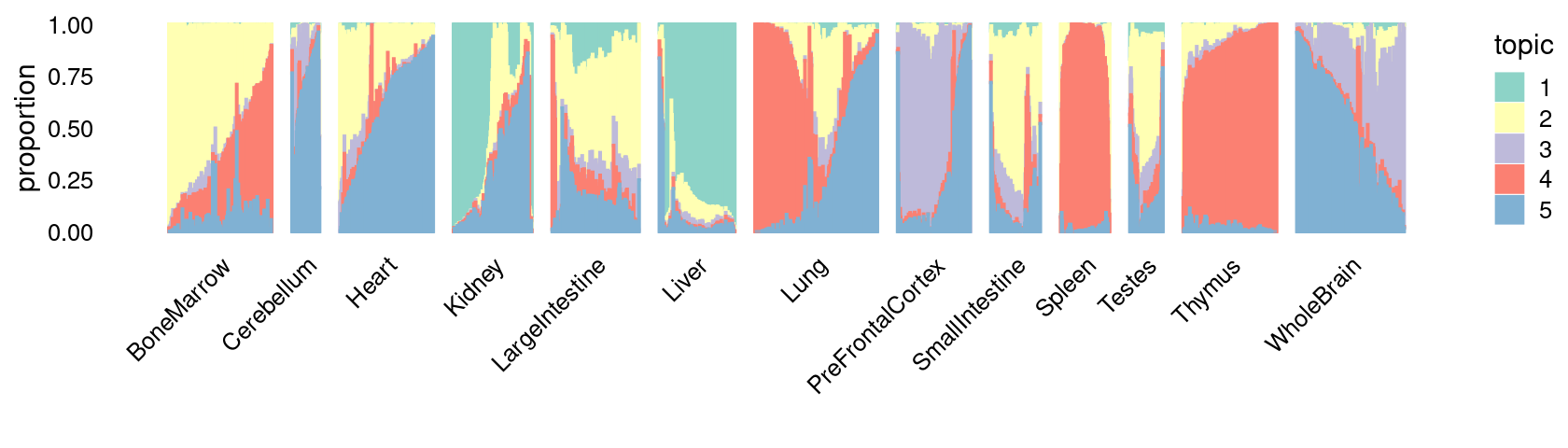
| Version | Author | Date |
|---|---|---|
| 5a8479b | kevinlkx | 2020-09-10 |
\(k = 6\):
fit_poisson_nmf <- fits[["fit-Cusanovich2018-scd-ex-k=6"]]

p.structure_plot <- structure_plot(poisson2multinom(fit_poisson_nmf),
                     grouping = samples[,"tissue"],
                     n = 2000,gap = 40,num_threads = 4,verbose = FALSE)
print(p.structure_plot)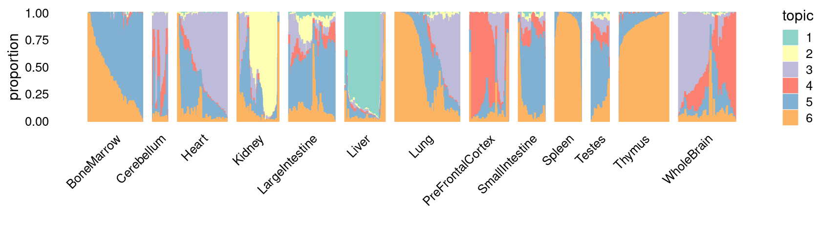
| Version | Author | Date |
|---|---|---|
| 5a8479b | kevinlkx | 2020-09-10 |
\(k = 7\):
fit_poisson_nmf <- fits[["fit-Cusanovich2018-scd-ex-k=7"]]

p.structure_plot <- structure_plot(poisson2multinom(fit_poisson_nmf),
                     grouping = samples[,"tissue"],
                     n = 2000,gap = 40,num_threads = 4,verbose = FALSE)
print(p.structure_plot)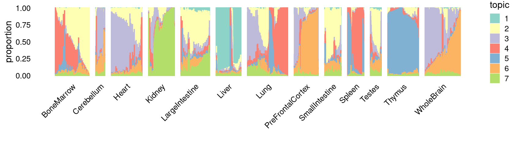
| Version | Author | Date |
|---|---|---|
| 5a8479b | kevinlkx | 2020-09-10 |
\(k = 8\):
fit_poisson_nmf <- fits[["fit-Cusanovich2018-scd-ex-k=8"]]

p.structure_plot <- structure_plot(poisson2multinom(fit_poisson_nmf),
                     grouping = samples[,"tissue"],
                     n = 2000,gap = 40,num_threads = 4,verbose = FALSE)
print(p.structure_plot)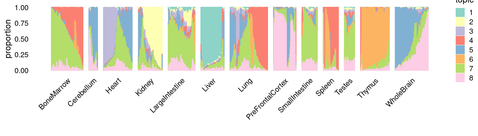
| Version | Author | Date |
|---|---|---|
| 5a8479b | kevinlkx | 2020-09-10 |
\(k = 9\):
fit_poisson_nmf <- fits[["fit-Cusanovich2018-scd-ex-k=9"]]

p.structure_plot <- structure_plot(poisson2multinom(fit_poisson_nmf),
                     grouping = samples[,"tissue"],
                     n = 2000,gap = 40,num_threads = 4,verbose = FALSE)
print(p.structure_plot)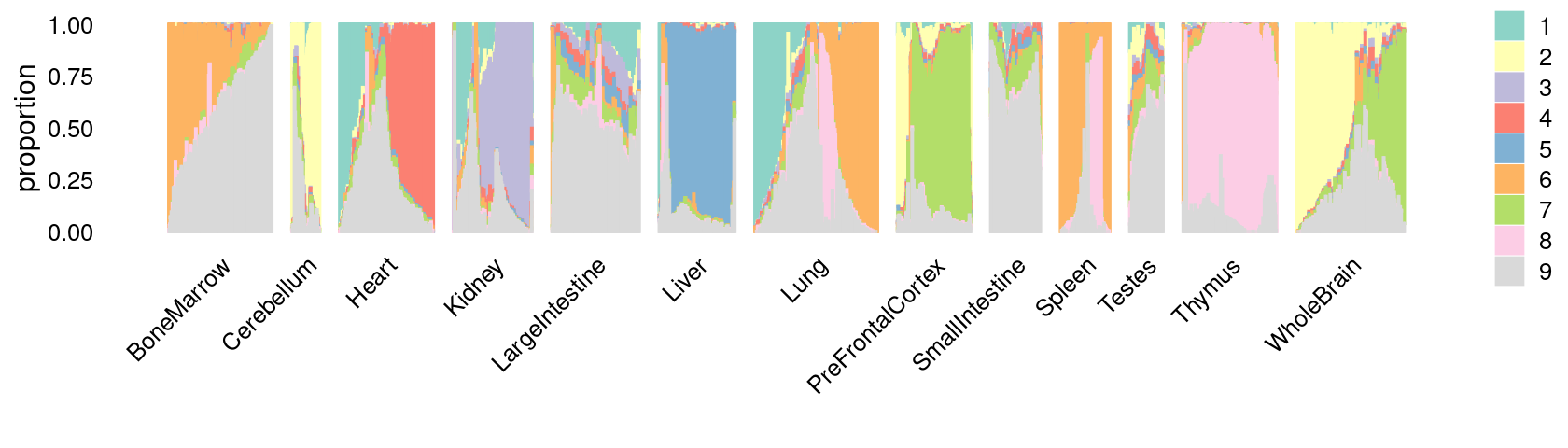
| Version | Author | Date |
|---|---|---|
| 5a8479b | kevinlkx | 2020-09-10 |
\(k = 10\):
fit_poisson_nmf <- fits[["fit-Cusanovich2018-scd-ex-k=10"]]

p.structure_plot <- structure_plot(poisson2multinom(fit_poisson_nmf),
                     grouping = samples[,"tissue"],
                     n = 2000,gap = 40,num_threads = 4,verbose = FALSE)
print(p.structure_plot)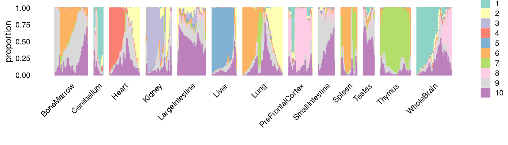
| Version | Author | Date |
|---|---|---|
| 5a8479b | kevinlkx | 2020-09-10 |
t-SNE plot
Plot samples by tissues on the t-SNE coordinates provided by the original paper:
p.tissues_tsne <- ggplot(samples, aes(x = tsne_1, y = tsne_2)) +
  geom_point(aes(colour = tissue), size = 0.5) +
  labs(x = 't-SNE 1', y = 't-SNE 2', title = '') +
  scale_color_discrete('') +
  theme_classic()

print(p.tissues_tsne)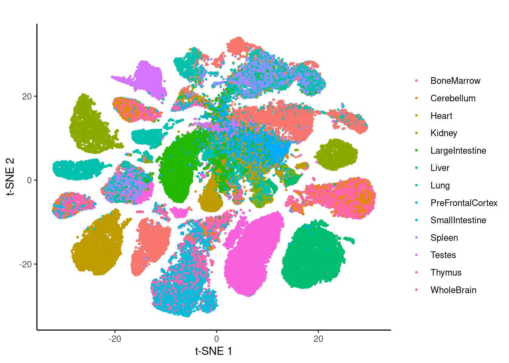
| Version | Author | Date |
|---|---|---|
| 7c0b14f | kevinlkx | 2020-09-11 |
Plot a random subset of 2000 samples by tissues:
idx_plot <- sort(sample(1:length(samples$cell), 2000))

p.tissues_tsne <- ggplot(samples[idx_plot,], aes(x = tsne_1, y = tsne_2)) +
  geom_point(aes(colour = tissue), size = 0.5) +
  labs(x = 't-SNE 1', y = 't-SNE 2', title = '') +
  scale_color_discrete('') +
  theme_classic()

print(p.tissues_tsne)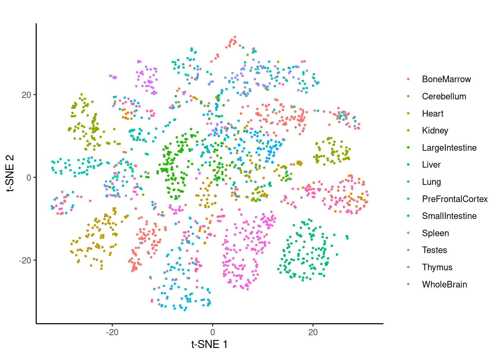
| Version | Author | Date |
|---|---|---|
| 7c0b14f | kevinlkx | 2020-09-11 |
Visualize topic membership using pie-charts on t-SNE coordinates
Visualize topic membership using pie-charts for cells on t-SNE coordinates provided by the original paper
Plot the subset of 2000 samples:
\(k = 3\):
k <- 3
fit_poisson_nmf <- fits[[sprintf("fit-Cusanovich2018-scd-ex-k=%d", k)]]
fit <- poisson2multinom(fit_poisson_nmf)

plot(NA,NA, main = paste("K =", k),
     xlab = 't-SNE 1', ylab = 't-SNE 2',
     xlim=c(min(samples$tsne_1),max(samples$tsne_1)),
     ylim=c(min(samples$tsne_2),max(samples$tsne_2)))

res <- lapply(idx_plot, function(r)
  add.pie(z=as.integer(100*fit$L[r,]),
          x=samples[r,"tsne_1"],
          y=samples[r,"tsne_2"], labels=c("","",""),
          radius = 1, col = RColorBrewer::brewer.pal(9, "Set1")))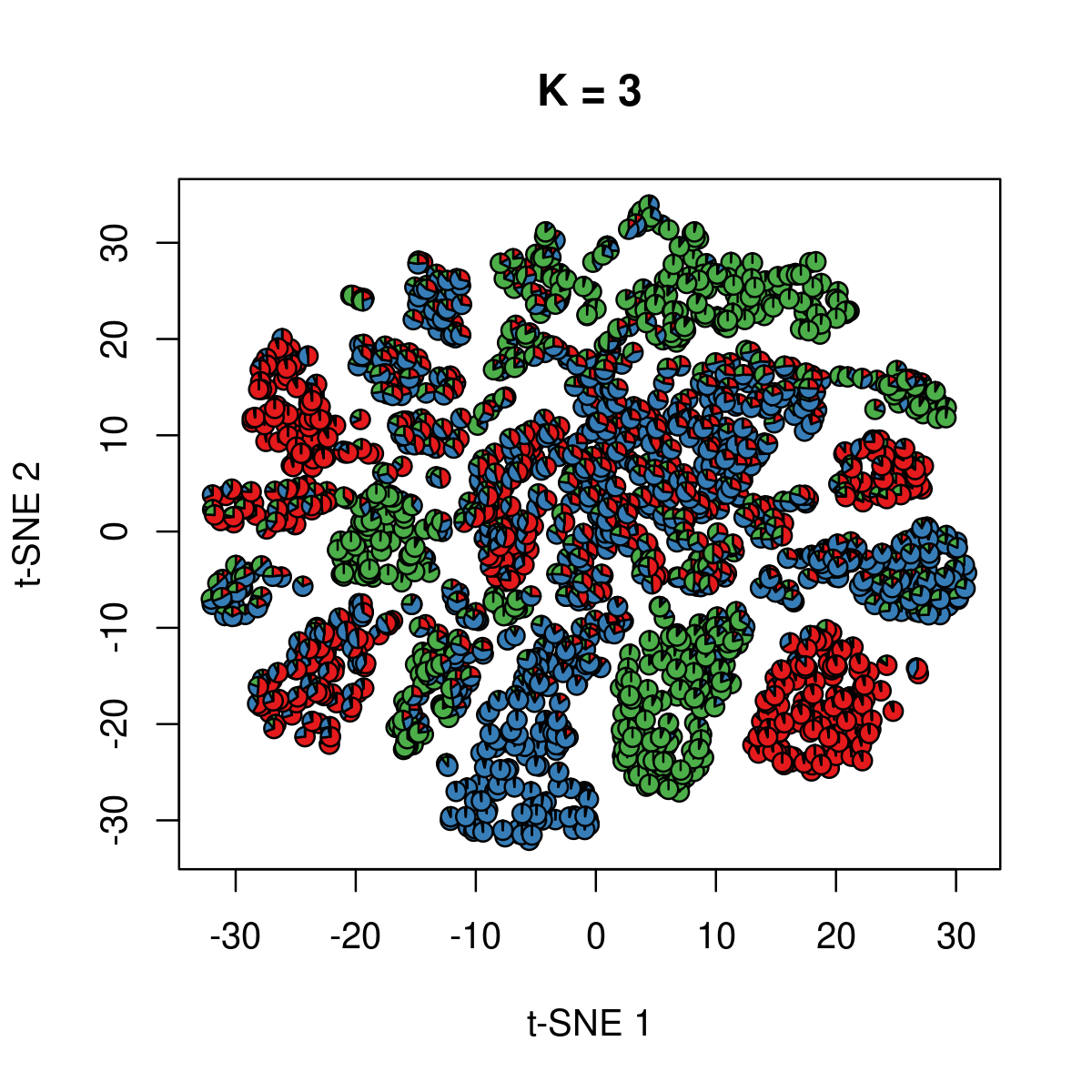
| Version | Author | Date |
|---|---|---|
| 7c0b14f | kevinlkx | 2020-09-11 |
\(k = 4\):
k <- 4
fit_poisson_nmf <- fits[[sprintf("fit-Cusanovich2018-scd-ex-k=%d", k)]]
fit <- poisson2multinom(fit_poisson_nmf)

plot(NA,NA, main = paste("K =", k),
     xlab = 't-SNE 1', ylab = 't-SNE 2',
     xlim=c(min(samples$tsne_1),max(samples$tsne_1)),
     ylim=c(min(samples$tsne_2),max(samples$tsne_2)))

res <- lapply(idx_plot, function(r)
  add.pie(z=as.integer(100*fit$L[r,]),
          x=samples[r,"tsne_1"],
          y=samples[r,"tsne_2"], labels=c("","",""),
          radius = 1, col = RColorBrewer::brewer.pal(9, "Set1")))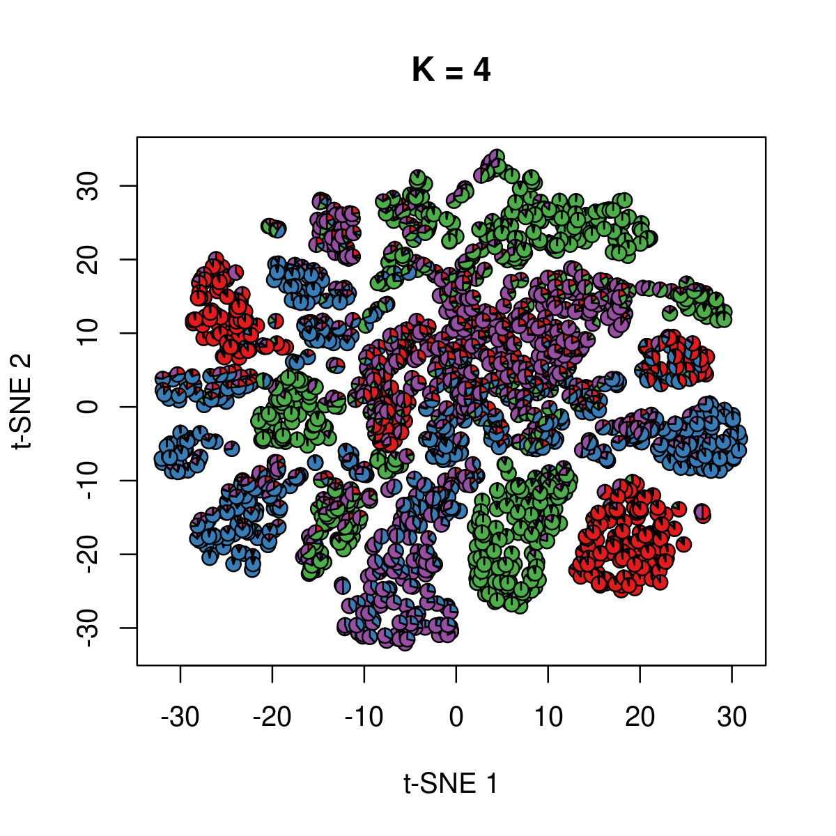
| Version | Author | Date |
|---|---|---|
| 7c0b14f | kevinlkx | 2020-09-11 |
\(k = 5\):
k <- 5
fit_poisson_nmf <- fits[[sprintf("fit-Cusanovich2018-scd-ex-k=%d", k)]]
fit <- poisson2multinom(fit_poisson_nmf)

plot(NA,NA, main = paste("K =", k),
     xlab = 't-SNE 1', ylab = 't-SNE 2',
     xlim=c(min(samples$tsne_1),max(samples$tsne_1)),
     ylim=c(min(samples$tsne_2),max(samples$tsne_2)))

res <- lapply(idx_plot, function(r)
  add.pie(z=as.integer(100*fit$L[r,]),
          x=samples[r,"tsne_1"],
          y=samples[r,"tsne_2"], labels=c("","",""),
          radius = 1, col = RColorBrewer::brewer.pal(9, "Set1")))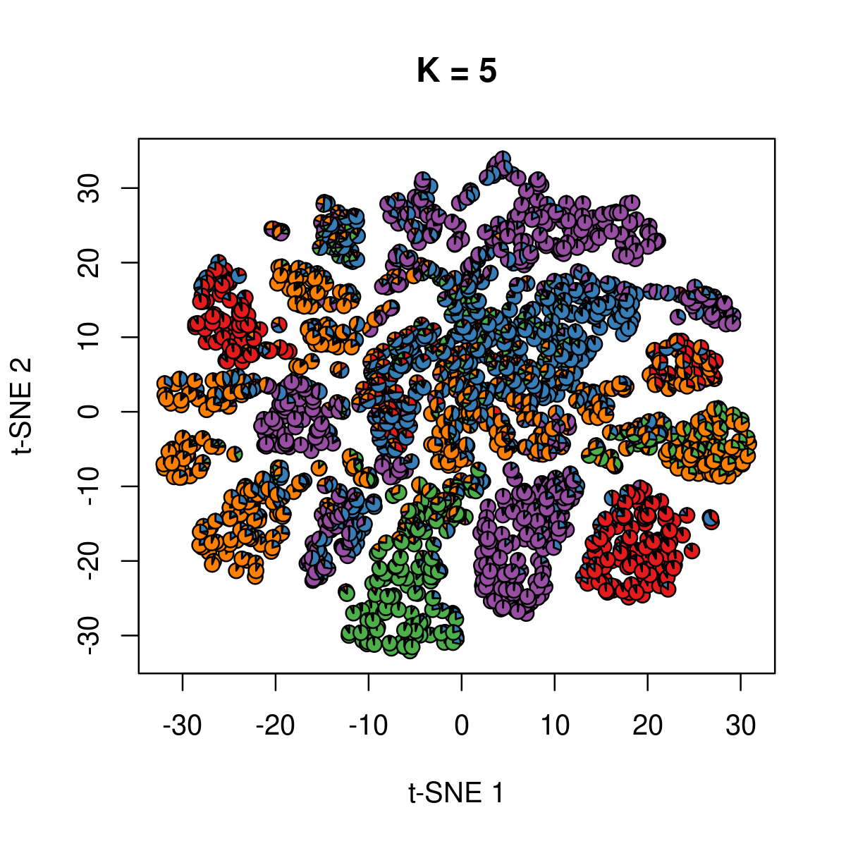
| Version | Author | Date |
|---|---|---|
| 7c0b14f | kevinlkx | 2020-09-11 |
\(k = 6\):
k <- 6
fit_poisson_nmf <- fits[[sprintf("fit-Cusanovich2018-scd-ex-k=%d", k)]]
fit <- poisson2multinom(fit_poisson_nmf)

plot(NA,NA, main = paste("K =", k),
     xlab = 't-SNE 1', ylab = 't-SNE 2',
     xlim=c(min(samples$tsne_1),max(samples$tsne_1)),
     ylim=c(min(samples$tsne_2),max(samples$tsne_2)))

res <- lapply(idx_plot, function(r)
  add.pie(z=as.integer(100*fit$L[r,]),
          x=samples[r,"tsne_1"],
          y=samples[r,"tsne_2"], labels=c("","",""),
          radius = 1, col = RColorBrewer::brewer.pal(9, "Set1")))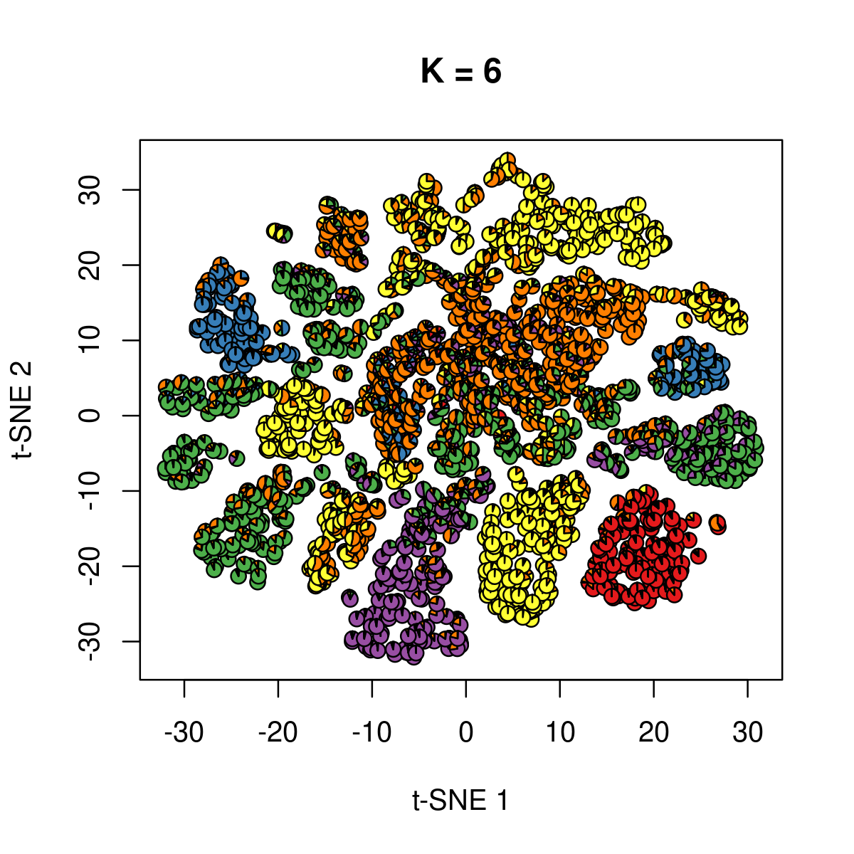
| Version | Author | Date |
|---|---|---|
| 7c0b14f | kevinlkx | 2020-09-11 |
\(k = 7\):
k <- 7
fit_poisson_nmf <- fits[[sprintf("fit-Cusanovich2018-scd-ex-k=%d", k)]]
fit <- poisson2multinom(fit_poisson_nmf)

plot(NA,NA, main = paste("K =", k),
     xlab = 't-SNE 1', ylab = 't-SNE 2',
     xlim=c(min(samples$tsne_1),max(samples$tsne_1)),
     ylim=c(min(samples$tsne_2),max(samples$tsne_2)))

res <- lapply(idx_plot, function(r)
  add.pie(z=as.integer(100*fit$L[r,]),
          x=samples[r,"tsne_1"],
          y=samples[r,"tsne_2"], labels=c("","",""),
          radius = 1, col = RColorBrewer::brewer.pal(9, "Set1")))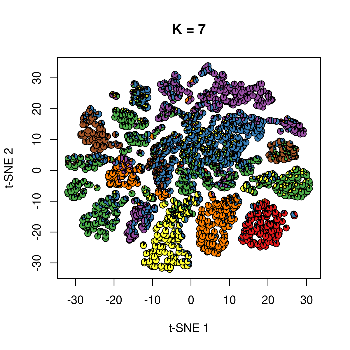
| Version | Author | Date |
|---|---|---|
| 7c0b14f | kevinlkx | 2020-09-11 |
\(k = 8\):
k <- 8
fit_poisson_nmf <- fits[[sprintf("fit-Cusanovich2018-scd-ex-k=%d", k)]]
fit <- poisson2multinom(fit_poisson_nmf)

plot(NA,NA, main = paste("K =", k),
     xlab = 't-SNE 1', ylab = 't-SNE 2',
     xlim=c(min(samples$tsne_1),max(samples$tsne_1)),
     ylim=c(min(samples$tsne_2),max(samples$tsne_2)))

res <- lapply(idx_plot, function(r)
  add.pie(z=as.integer(100*fit$L[r,]),
          x=samples[r,"tsne_1"],
          y=samples[r,"tsne_2"], labels=c("","",""),
          radius = 1, col = RColorBrewer::brewer.pal(9, "Set1")))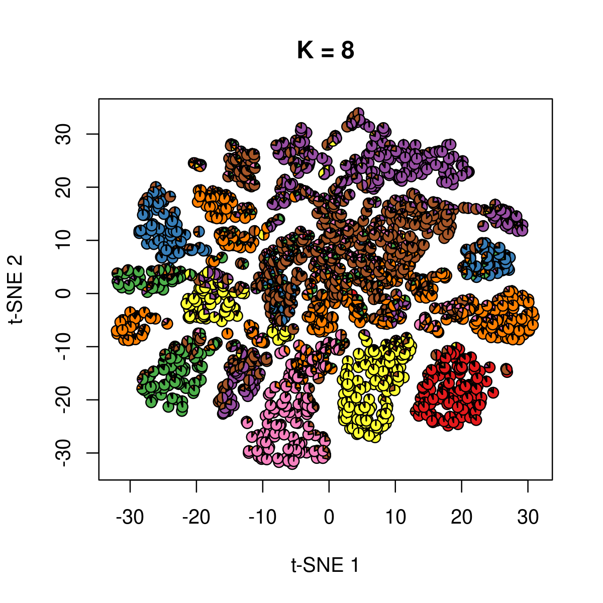
| Version | Author | Date |
|---|---|---|
| 7c0b14f | kevinlkx | 2020-09-11 |
\(k = 9\):
k <- 9
fit_poisson_nmf <- fits[[sprintf("fit-Cusanovich2018-scd-ex-k=%d", k)]]
fit <- poisson2multinom(fit_poisson_nmf)

plot(NA,NA, main = paste("K =", k),
     xlab = 't-SNE 1', ylab = 't-SNE 2',
     xlim=c(min(samples$tsne_1),max(samples$tsne_1)),
     ylim=c(min(samples$tsne_2),max(samples$tsne_2)))

res <- lapply(idx_plot, function(r)
  add.pie(z=as.integer(100*fit$L[r,]),
          x=samples[r,"tsne_1"],
          y=samples[r,"tsne_2"], labels=c("","",""),
          radius = 1, col = RColorBrewer::brewer.pal(9, "Set1")))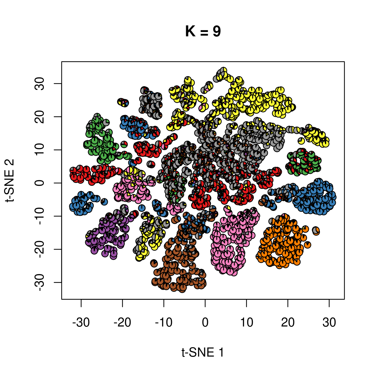
| Version | Author | Date |
|---|---|---|
| 7c0b14f | kevinlkx | 2020-09-11 |
\(k = 10\):
k <- 10
fit_poisson_nmf <- fits[[sprintf("fit-Cusanovich2018-scd-ex-k=%d", k)]]
fit <- poisson2multinom(fit_poisson_nmf)

plot(NA,NA, main = paste("K =", k),
     xlab = 't-SNE 1', ylab = 't-SNE 2',
     xlim=c(min(samples$tsne_1),max(samples$tsne_1)),
     ylim=c(min(samples$tsne_2),max(samples$tsne_2)))

res <- lapply(idx_plot, function(r)
  add.pie(z=as.integer(100*fit$L[r,]),
          x=samples[r,"tsne_1"],
          y=samples[r,"tsne_2"], labels=c("","",""),
          radius = 1, col = RColorBrewer::brewer.pal(9, "Set1")))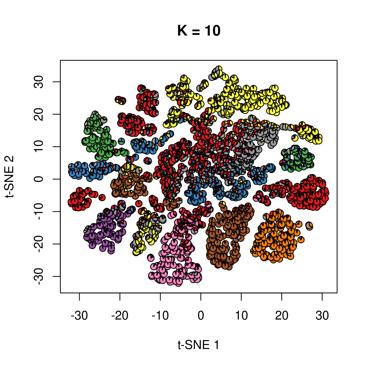
sessionInfo()
# R version 3.5.1 (2018-07-02)
# Platform: x86_64-pc-linux-gnu (64-bit)
# Running under: Scientific Linux 7.4 (Nitrogen)
#
# Matrix products: default
# BLAS/LAPACK: /software/openblas-0.2.19-el7-x86_64/lib/libopenblas_haswellp-r0.2.19.so
#
# locale:
#  [1] LC_CTYPE=en_US.UTF-8       LC_NUMERIC=C
#  [3] LC_TIME=en_US.UTF-8        LC_COLLATE=en_US.UTF-8
#  [5] LC_MONETARY=en_US.UTF-8    LC_MESSAGES=en_US.UTF-8
#  [7] LC_PAPER=en_US.UTF-8       LC_NAME=C
#  [9] LC_ADDRESS=C               LC_TELEPHONE=C
# [11] LC_MEASUREMENT=en_US.UTF-8 LC_IDENTIFICATION=C
#
# attached base packages:
# [1] tools     stats     graphics  grDevices utils     datasets  methods
# [8] base
#
# other attached packages:
# [1] mapplots_1.5.1     cowplot_1.0.0      ggplot2_3.3.0      fastTopics_0.3-163
# [5] dplyr_0.8.5        workflowr_1.6.2
#
# loaded via a namespace (and not attached):
#  [1] ggrepel_0.8.2      Rcpp_1.0.4.6       lattice_0.20-38    tidyr_0.8.3
#  [5] prettyunits_1.1.1  assertthat_0.2.1   rprojroot_1.3-2    digest_0.6.25
#  [9] R6_2.4.1           backports_1.1.7    MatrixModels_0.4-1 evaluate_0.14
# [13] coda_0.19-2        httr_1.4.1         pillar_1.4.4       rlang_0.4.6
# [17] progress_1.2.2     lazyeval_0.2.2     data.table_1.12.8  irlba_2.3.3
# [21] SparseM_1.77       whisker_0.4        Matrix_1.2-15      rmarkdown_2.1
# [25] labeling_0.3       Rtsne_0.15         stringr_1.4.0      htmlwidgets_1.5.1
# [29] munsell_0.5.0      compiler_3.5.1     httpuv_1.5.3.1     xfun_0.14
# [33] pkgconfig_2.0.3    mcmc_0.9-7         htmltools_0.4.0    tidyselect_0.2.5
# [37] tibble_3.0.1       quadprog_1.5-5     viridisLite_0.3.0  crayon_1.3.4
# [41] withr_2.1.2        later_1.0.0        MASS_7.3-51.6      grid_3.5.1
# [45] jsonlite_1.6       gtable_0.3.0       lifecycle_0.2.0    git2r_0.27.1
# [49] magrittr_1.5       scales_1.1.1       RcppParallel_4.4.3 stringi_1.4.6
# [53] farver_2.0.3       fs_1.3.1           promises_1.1.0     ellipsis_0.3.1
# [57] vctrs_0.3.0        RColorBrewer_1.1-2 glue_1.4.1         purrr_0.3.4
# [61] hms_0.4.2          yaml_2.2.0         colorspace_1.4-1   plotly_4.8.0
# [65] knitr_1.28         quantreg_5.36      MCMCpack_1.4-4