Clustering Buenrostro et al (2018) scATAC-seq data using topic proportions with K = 11
Kaixuan Luo
Last updated: 2020-12-02
Checks: 7 0
Knit directory: scATACseq-topics/
This reproducible R Markdown analysis was created with workflowr (version 1.6.2). The Checks tab describes the reproducibility checks that were applied when the results were created. The Past versions tab lists the development history.
Great! Since the R Markdown file has been committed to the Git repository, you know the exact version of the code that produced these results.
Great job! The global environment was empty. Objects defined in the global environment can affect the analysis in your R Markdown file in unknown ways. For reproduciblity it's best to always run the code in an empty environment.
The command set.seed(20200729) was run prior to running the code in the R Markdown file. Setting a seed ensures that any results that rely on randomness, e.g. subsampling or permutations, are reproducible.
Great job! Recording the operating system, R version, and package versions is critical for reproducibility.
Nice! There were no cached chunks for this analysis, so you can be confident that you successfully produced the results during this run.
Great job! Using relative paths to the files within your workflowr project makes it easier to run your code on other machines.
Great! You are using Git for version control. Tracking code development and connecting the code version to the results is critical for reproducibility.
The results in this page were generated with repository version 6f28b44. See the Past versions tab to see a history of the changes made to the R Markdown and HTML files.
Note that you need to be careful to ensure that all relevant files for the analysis have been committed to Git prior to generating the results (you can use wflow_publish or wflow_git_commit). workflowr only checks the R Markdown file, but you know if there are other scripts or data files that it depends on. Below is the status of the Git repository when the results were generated:
Ignored files:
    Ignored:    .Rhistory
    Ignored:    .Rproj.user/

Untracked files:
    Untracked:  analysis/clusters_pca_structure_Cusanovich2018.Rmd
    Untracked:  analysis/motif_analysis_Buenrostro2018_chomVAR_scPeaks.Rmd
    Untracked:  analysis/process_data_Buenrostro2018_Chen2019.Rmd
    Untracked:  buenrostro2018.RData
    Untracked:  output/clustering-Cusanovich2018.rds
    Untracked:  scripts/fit_all_models_Buenrostro_2018_chromVar_scPeaks_filtered.sbatch

Unstaged changes:
    Modified:   analysis/cisTopic_Buenrostro2018_chomVAR_scPeaks.Rmd
    Modified:   analysis/plots_Lareau2019_bonemarrow.Rmd
    Modified:   analysis/process_data_Buenrostro2018.Rmd
    Modified:   code/motif_analysis.R
    Modified:   code/plots.R
    Modified:   scripts/fit_all_models_Buenrostro_2018.sbatch
Note that any generated files, e.g. HTML, png, CSS, etc., are not included in this status report because it is ok for generated content to have uncommitted changes.
These are the previous versions of the repository in which changes were made to the R Markdown (analysis/clusters_Buenrostro2018_k11_Chen2019pipeline.Rmd) and HTML (docs/clusters_Buenrostro2018_k11_Chen2019pipeline.html) files. If you've configured a remote Git repository (see ?wflow_git_remote), click on the hyperlinks in the table below to view the files as they were in that past version.
| File | Version | Author | Date | Message |
|---|---|---|---|---|
| Rmd | 6f28b44 | kevinlkx | 2020-12-02 | update data.dir and out.dir |
| Rmd | 6a9dead | kevinlkx | 2020-11-19 | wflow_rename("analysis/clusters_Buenrostro2018_k11.Rmd", "analysis/clusters_Buenrostro2018_k11_Chen2019pipeline.Rmd") |
| html | 6a9dead | kevinlkx | 2020-11-19 | wflow_rename("analysis/clusters_Buenrostro2018_k11.Rmd", "analysis/clusters_Buenrostro2018_k11_Chen2019pipeline.Rmd") |
Here we explore the structure in the Buenrostro et al (2018) scATAC-seq data inferred from the multinomial topic model with \(k = 11\).
Load packages and some functions used in this analysis.
library(Matrix)
library(dplyr)
library(ggplot2)
library(cowplot)
library(fastTopics)
source("code/plots.R")
We applied the analysis both unbinarized counts and binarized scATAC-seq data.
Unbinarized counts
Load the unbinarized data
data.dir <- "/project2/mstephens/kevinluo/scATACseq-topics/data/Buenrostro_2018/processed_data_Chen2019pipeline/"
load(file.path(data.dir, "Buenrostro_2018_counts.RData"))
cat(sprintf("%d x %d counts matrix.\n",nrow(counts),ncol(counts)))
rm(counts)
samples$cell <- rownames(samples)
samples$label <- as.factor(samples$label)
# 2034 x 101172 counts matrix.
Plot PCs of the topic proportions
We first use PCA to explore the structure inferred from the multinomial topic model with \(k = 11\):
out.dir <- "/project2/mstephens/kevinluo/scATACseq-topics/output/Buenrostro_2018_Chen2019pipeline/unbinarized/"
fit <- readRDS(file.path(out.dir, "/fit-Buenrostro2018-scd-ex-k=11.rds"))$fit

colors_topics <- c("#a6cee3","#1f78b4","#b2df8a","#33a02c","#fb9a99","#e31a1c",
                   "#fdbf6f","#ff7f00","#cab2d6","#6a3d9a","#ffff99")
Plot PCs of the topic proportions.
p.pca1.1 <- pca_plot(poisson2multinom(fit),pcs = 1:2,fill = "none")
p.pca1.2 <- pca_plot(poisson2multinom(fit),pcs = 3:4,fill = "none")
p.pca1.3 <- pca_plot(poisson2multinom(fit),pcs = 5:6,fill = "none")
p.pca1.4 <- pca_plot(poisson2multinom(fit),pcs = 7:8,fill = "none")
p.pca1.5 <- pca_plot(poisson2multinom(fit),pcs = 9:10,fill = "none")

plot_grid(p.pca1.1,p.pca1.2,p.pca1.3,p.pca1.4,p.pca1.5)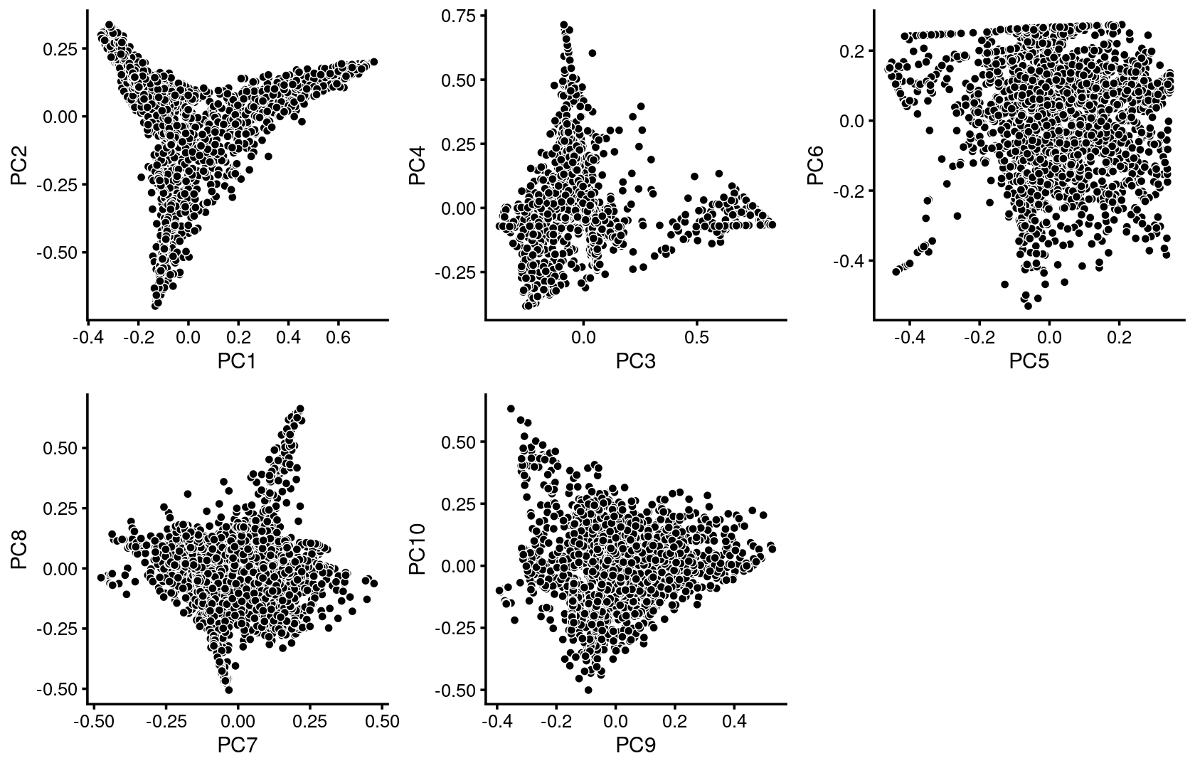
| Version | Author | Date |
|---|---|---|
| 6a9dead | kevinlkx | 2020-11-19 |
Some of the structure is more evident from “hexbin” plots showing the density of the points.
breaks <- c(0,1,5,10,100,Inf)
p.pca2.1 <- pca_hexbin_plot(poisson2multinom(fit), pcs = 1:2, breaks = breaks) + guides(fill = "none")
p.pca2.2 <- pca_hexbin_plot(poisson2multinom(fit), pcs = 3:4, breaks = breaks) + guides(fill = "none")
p.pca2.3 <- pca_hexbin_plot(poisson2multinom(fit), pcs = 5:6, breaks = breaks) + guides(fill = "none")
p.pca2.4 <- pca_hexbin_plot(poisson2multinom(fit), pcs = 7:8, breaks = breaks) + guides(fill = "none")
p.pca2.5 <- pca_hexbin_plot(poisson2multinom(fit), pcs = 9:10, breaks = breaks) + guides(fill = "none")

plot_grid(p.pca2.1,p.pca2.2,p.pca2.3,p.pca2.4,p.pca2.5)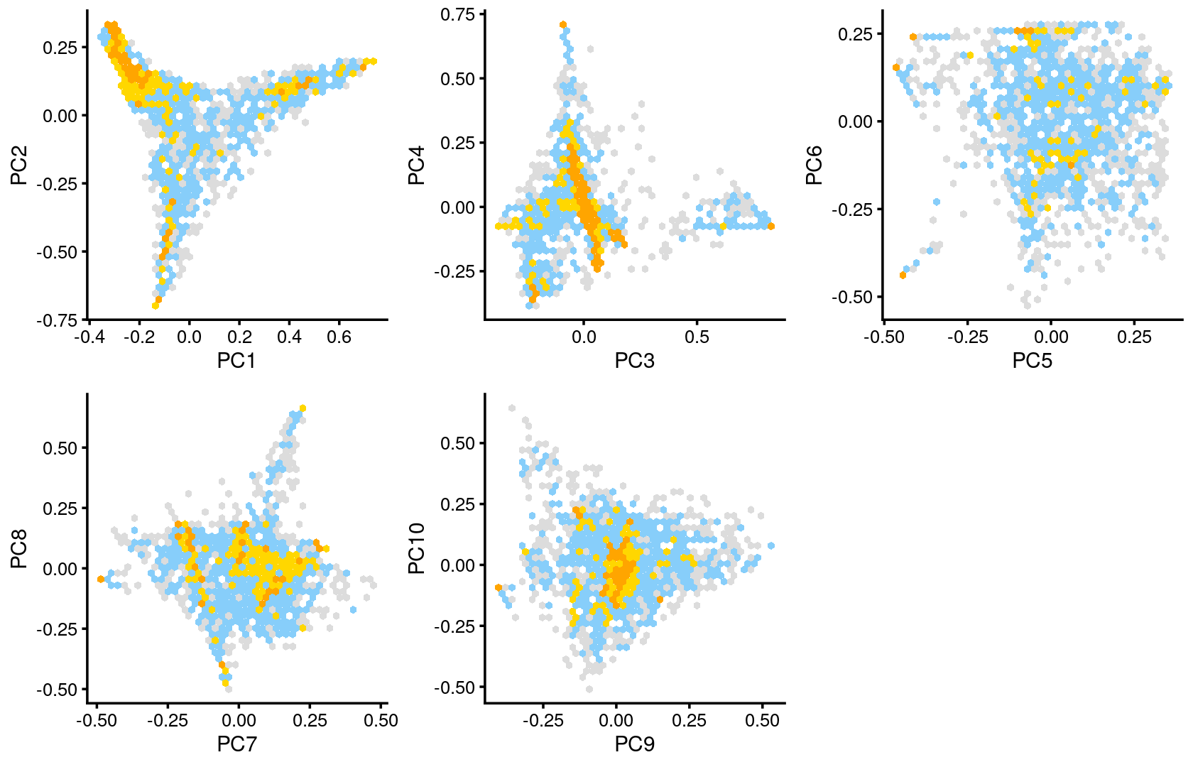
| Version | Author | Date |
|---|---|---|
| 6a9dead | kevinlkx | 2020-11-19 |
Layer the cell labels onto the PC plots
Here, we layer the cell labels onto the PC plots.
p.pca3.1 <- labeled_pca_plot(fit,1:2,samples$label,font_size = 7,
                       legend_label = "Cell labels")
p.pca3.2 <- labeled_pca_plot(fit,3:4,samples$label,font_size = 7,
                       legend_label = "Cell labels")
p.pca3.3 <- labeled_pca_plot(fit,5:6,samples$label,font_size = 7,
                       legend_label = "Cell labels")
p.pca3.4 <- labeled_pca_plot(fit,7:8,samples$label,font_size = 7,
                       legend_label = "Cell labels")
p.pca3.5 <- labeled_pca_plot(fit,9:10,samples$label,font_size = 7,
                       legend_label = "Cell labels")
plot_grid(p.pca3.1,p.pca3.2,p.pca3.3,p.pca3.4,p.pca3.5)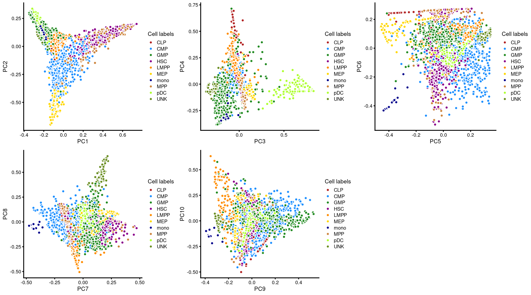
| Version | Author | Date |
|---|---|---|
| 6a9dead | kevinlkx | 2020-11-19 |
Visualize by structure plot grouped by cell labels.
set.seed(10)

samples$label <- as.factor(samples$label)

p.structure.1 <- structure_plot(poisson2multinom(fit),
                     grouping = samples[, "label"],n = Inf,gap = 20,
                     perplexity = 50,topics = 1:11,colors = colors_topics,
                     num_threads = 4,verbose = FALSE)
# Perplexity automatically changed to 24 because original setting of 50 was too large for the number of samples (78)
# Perplexity automatically changed to 44 because original setting of 50 was too large for the number of samples (138)
# Perplexity automatically changed to 20 because original setting of 50 was too large for the number of samples (64)
# Perplexity automatically changed to 46 because original setting of 50 was too large for the number of samples (142)
# Perplexity automatically changed to 45 because original setting of 50 was too large for the number of samples (141)
# Perplexity automatically changed to 18 because original setting of 50 was too large for the number of samples (60)

print(p.structure.1)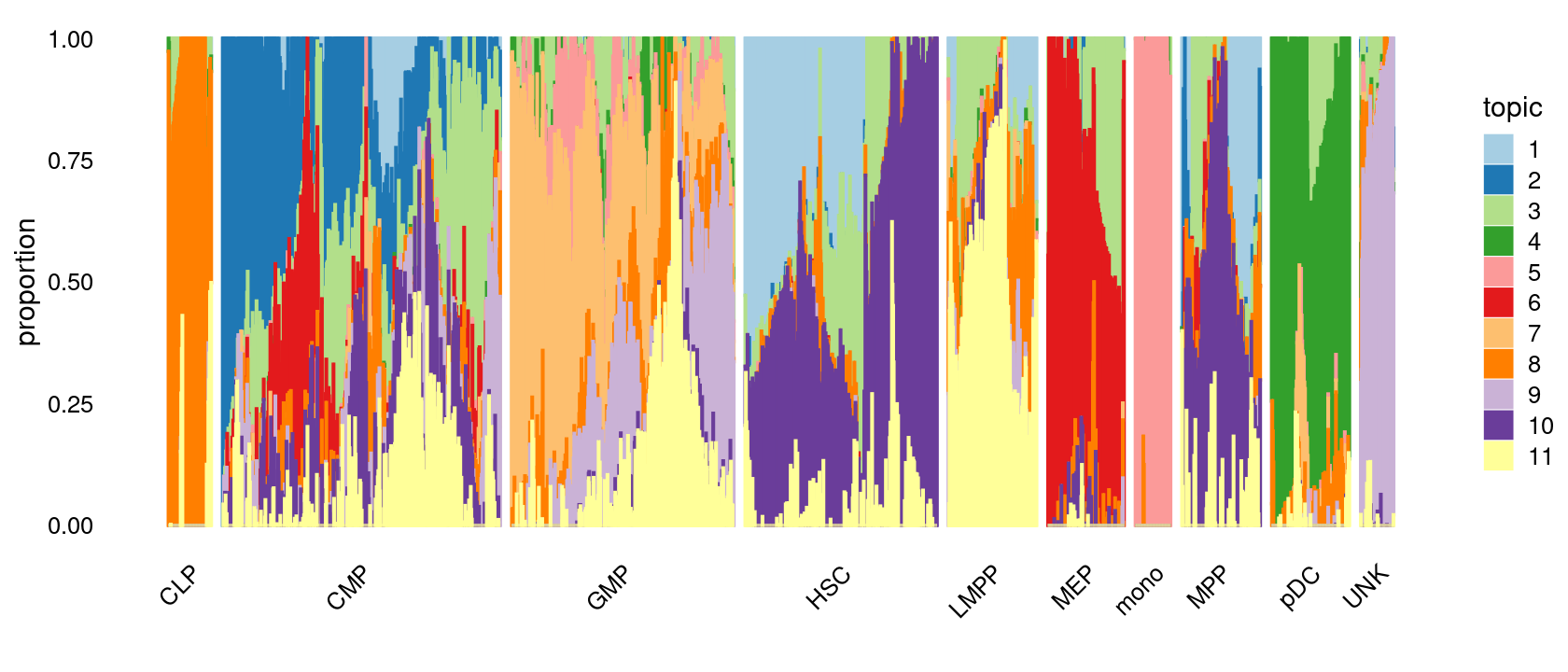
| Version | Author | Date |
|---|---|---|
| 6a9dead | kevinlkx | 2020-11-19 |
k-means clustering on topic proportions
Define clusters using k-means, and then create structure plot based on the clusters from k-means.
Define clusters using k-means with \(k = 10\):
set.seed(10)

clusters.10 <- factor(kmeans(poisson2multinom(fit)$L,centers = 10)$cluster)
print(sort(table(clusters.10),decreasing = TRUE))
# clusters.10
#   1   5   4  10   7   2   8   9   6   3
# 401 300 249 233 226 166 166 143  84  66
Structure plot based on k-means clusters
p.structure.2 <- structure_plot(poisson2multinom(fit),
                     grouping = clusters.10,
                     # rows = order(samples$label), # samples are grouped by clusters first, then by celltype labels
                     n = Inf,gap = 20,
                     perplexity = 50,topics = 1:11,colors = colors_topics,
                     num_threads = 4,verbose = FALSE)
# Perplexity automatically changed to 20 because original setting of 50 was too large for the number of samples (66)
# Perplexity automatically changed to 26 because original setting of 50 was too large for the number of samples (84)
# Perplexity automatically changed to 46 because original setting of 50 was too large for the number of samples (143)
print(p.structure.2)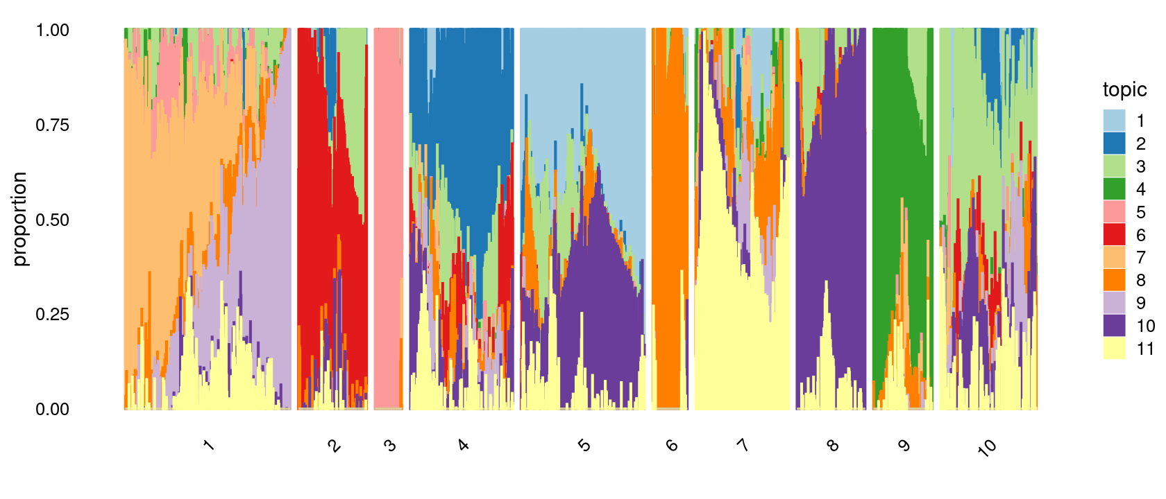
| Version | Author | Date |
|---|---|---|
| 6a9dead | kevinlkx | 2020-11-19 |
Define clusters using k-means with \(k = 15\):
set.seed(10)

clusters.15 <- factor(kmeans(poisson2multinom(fit)$L,centers = 15)$cluster)
print(sort(table(clusters.15),decreasing = TRUE))
# clusters.15
#   6  15   4  10   1   9   3  11   7   8  12   5   2  13  14
# 277 242 178 150 143 143 136 135 125 122 100  83  67  67  66
Structure plot based on k-means clusters
p.structure.3 <- structure_plot(poisson2multinom(fit),
                     grouping = clusters.15,
                     # rows = order(samples$label), # samples are grouped by clusters first, then by celltype labels
                     n = Inf,gap = 20,
                     perplexity = 50,topics = 1:11, colors = colors_topics,
                     num_threads = 4,verbose = FALSE)
# Perplexity automatically changed to 46 because original setting of 50 was too large for the number of samples (143)
# Perplexity automatically changed to 21 because original setting of 50 was too large for the number of samples (67)
# Perplexity automatically changed to 44 because original setting of 50 was too large for the number of samples (136)
# Perplexity automatically changed to 26 because original setting of 50 was too large for the number of samples (83)
# Perplexity automatically changed to 40 because original setting of 50 was too large for the number of samples (125)
# Perplexity automatically changed to 39 because original setting of 50 was too large for the number of samples (122)
# Perplexity automatically changed to 46 because original setting of 50 was too large for the number of samples (143)
# Perplexity automatically changed to 48 because original setting of 50 was too large for the number of samples (150)
# Perplexity automatically changed to 43 because original setting of 50 was too large for the number of samples (135)
# Perplexity automatically changed to 32 because original setting of 50 was too large for the number of samples (100)
# Perplexity automatically changed to 21 because original setting of 50 was too large for the number of samples (67)
# Perplexity automatically changed to 20 because original setting of 50 was too large for the number of samples (66)
print(p.structure.3)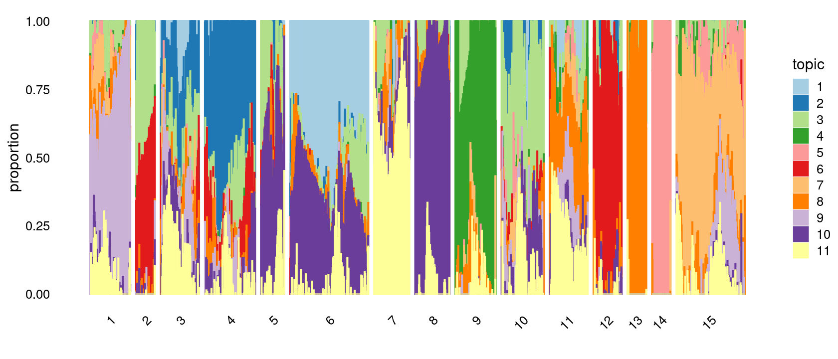
| Version | Author | Date |
|---|---|---|
| 6a9dead | kevinlkx | 2020-11-19 |
Define clusters using k-means with \(k = 20\):
set.seed(10)

clusters.20 <- factor(kmeans(poisson2multinom(fit)$L,centers = 20)$cluster)
print(sort(table(clusters.20),decreasing = TRUE))
# clusters.20
#  20   9  18   4  14   6   7  11  16  15   8  10  12   1   3  13  17   2   5  19
# 185 141 139 136 131 121 114 112 111 109 107  98  78  69  68  66  66  65  59  59
Structure plot based on k-means clusters
p.structure.4 <- structure_plot(poisson2multinom(fit),
                     grouping = clusters.20,
                     # rows = order(samples$label), # samples are grouped by clusters first, then by celltype labels
                     n = Inf,gap = 20,
                     perplexity = 50,topics = 1:11, colors = colors_topics,
                     num_threads = 4,verbose = FALSE)
# Perplexity automatically changed to 21 because original setting of 50 was too large for the number of samples (69)
# Perplexity automatically changed to 20 because original setting of 50 was too large for the number of samples (65)
# Perplexity automatically changed to 21 because original setting of 50 was too large for the number of samples (68)
# Perplexity automatically changed to 44 because original setting of 50 was too large for the number of samples (136)
# Perplexity automatically changed to 18 because original setting of 50 was too large for the number of samples (59)
# Perplexity automatically changed to 39 because original setting of 50 was too large for the number of samples (121)
# Perplexity automatically changed to 36 because original setting of 50 was too large for the number of samples (114)
# Perplexity automatically changed to 34 because original setting of 50 was too large for the number of samples (107)
# Perplexity automatically changed to 45 because original setting of 50 was too large for the number of samples (141)
# Perplexity automatically changed to 31 because original setting of 50 was too large for the number of samples (98)
# Perplexity automatically changed to 36 because original setting of 50 was too large for the number of samples (112)
# Perplexity automatically changed to 24 because original setting of 50 was too large for the number of samples (78)
# Perplexity automatically changed to 20 because original setting of 50 was too large for the number of samples (66)
# Perplexity automatically changed to 42 because original setting of 50 was too large for the number of samples (131)
# Perplexity automatically changed to 35 because original setting of 50 was too large for the number of samples (109)
# Perplexity automatically changed to 35 because original setting of 50 was too large for the number of samples (111)
# Perplexity automatically changed to 20 because original setting of 50 was too large for the number of samples (66)
# Perplexity automatically changed to 45 because original setting of 50 was too large for the number of samples (139)
# Perplexity automatically changed to 18 because original setting of 50 was too large for the number of samples (59)
print(p.structure.4)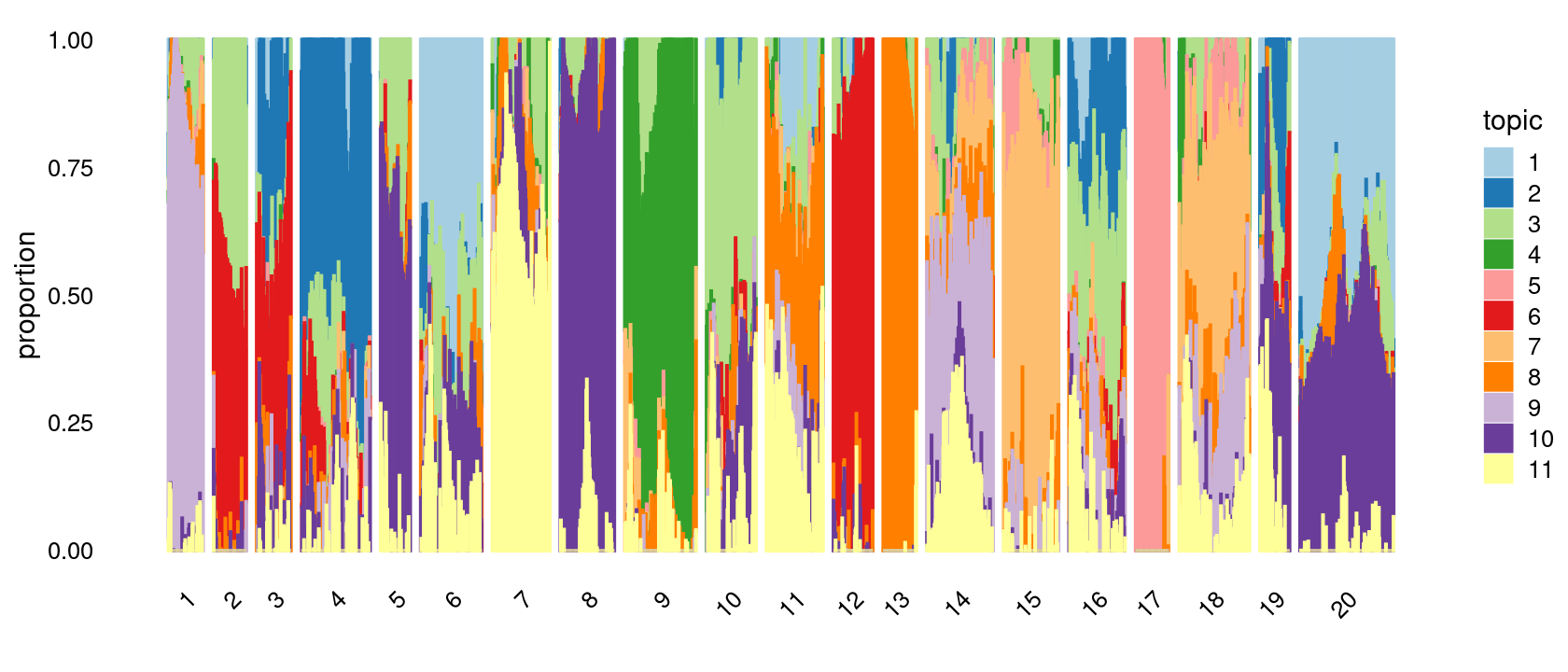
| Version | Author | Date |
|---|---|---|
| 6a9dead | kevinlkx | 2020-11-19 |
Refine clusters
We then further refine the clusters based on k-means result with \(k = 20\): merge clusters 5, 8; merge clusters 10 and 16; merge clusters 14 and 18.
clusters.merged <- clusters.20
clusters.merged[clusters.20 %in% c(5,8)] <- 5
clusters.merged[clusters.20 %in% c(10,16)] <- 10
clusters.merged[clusters.20 %in% c(14,18)] <- 14

clusters.merged <- factor(clusters.merged, labels = paste0("c", c(1:length(unique(clusters.merged)))))
samples$cluster_kmeans <- clusters.merged
table(clusters.merged)
# clusters.merged
#  c1  c2  c3  c4  c5  c6  c7  c8  c9 c10 c11 c12 c13 c14 c15 c16 c17
#  69  65  68 136 166 121 114 141 209 112  78  66 270 109  66  59 185
p.structure.refined <- structure_plot(poisson2multinom(fit),
grouping = clusters.merged,
# rows = order(samples$label), # samples are grouped by clusters first, then by celltype labels
n = Inf,gap = 20,
perplexity = 50,topics = 1:11,colors = colors_topics,
num_threads = 4,verbose = FALSE)
# Perplexity automatically changed to 21 because original setting of 50 was too large for the number of samples (69)
# Perplexity automatically changed to 20 because original setting of 50 was too large for the number of samples (65)
# Perplexity automatically changed to 21 because original setting of 50 was too large for the number of samples (68)
# Perplexity automatically changed to 44 because original setting of 50 was too large for the number of samples (136)
# Perplexity automatically changed to 39 because original setting of 50 was too large for the number of samples (121)
# Perplexity automatically changed to 36 because original setting of 50 was too large for the number of samples (114)
# Perplexity automatically changed to 45 because original setting of 50 was too large for the number of samples (141)
# Perplexity automatically changed to 36 because original setting of 50 was too large for the number of samples (112)
# Perplexity automatically changed to 24 because original setting of 50 was too large for the number of samples (78)
# Perplexity automatically changed to 20 because original setting of 50 was too large for the number of samples (66)
# Perplexity automatically changed to 35 because original setting of 50 was too large for the number of samples (109)
# Perplexity automatically changed to 20 because original setting of 50 was too large for the number of samples (66)
# Perplexity automatically changed to 18 because original setting of 50 was too large for the number of samples (59)
print(p.structure.refined)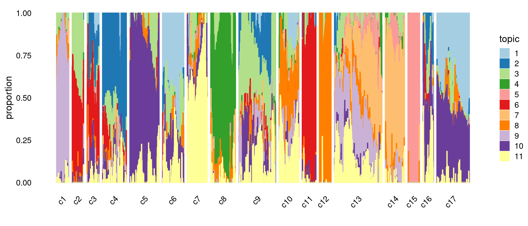
| Version | Author | Date |
|---|---|---|
| 6a9dead | kevinlkx | 2020-11-19 |
Group samples by k-means clusters first, then by celltype labels:
p.structure.refined <- structure_plot(poisson2multinom(fit),
                     grouping = clusters.merged,
                     rows = order(samples$label), # samples are grouped by clusters first, then by celltype labels
                     n = Inf,gap = 20,
                     perplexity = 50,topics = 1:11,colors = colors_topics,
                     num_threads = 4,verbose = FALSE)
print(p.structure.refined)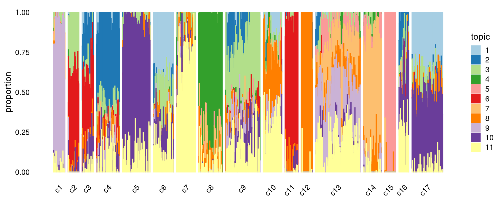
| Version | Author | Date |
|---|---|---|
| 6a9dead | kevinlkx | 2020-11-19 |
The clusters defined by k-means on topic proportions reasonably identify the clusters shown in the PCA hexbin plots (below).
p.pca.4.1 <- labeled_pca_plot(fit,1:2,samples$cluster_kmeans,font_size = 7,
                       legend_label = "cluster_kmeans")
p.pca.4.2 <- labeled_pca_plot(fit,3:4,samples$cluster_kmeans,font_size = 7,
                       legend_label = "cluster_kmeans")
p.pca.4.3 <- labeled_pca_plot(fit,5:6,samples$cluster_kmeans,font_size = 7,
                       legend_label = "cluster_kmeans")
p.pca.4.4 <- labeled_pca_plot(fit,7:8,samples$cluster_kmeans,font_size = 7,
                       legend_label = "cluster_kmeans")
p.pca.4.5 <- labeled_pca_plot(fit,9:10,samples$cluster_kmeans,font_size = 7,
                       legend_label = "cluster_kmeans")
plot_grid(p.pca.4.1,p.pca.4.2,p.pca.4.3,p.pca.4.4,p.pca.4.5)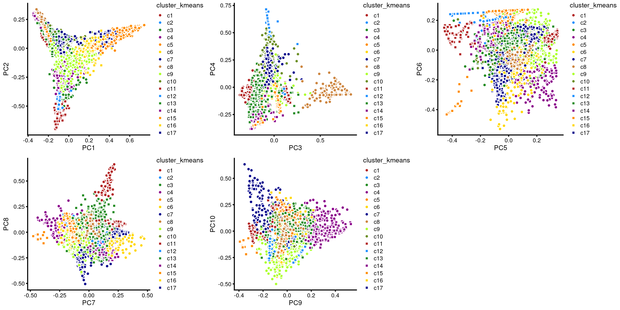
| Version | Author | Date |
|---|---|---|
| 6a9dead | kevinlkx | 2020-11-19 |
plot_grid(p.pca2.1,p.pca2.2,p.pca2.3,p.pca2.4,p.pca2.5)
| Version | Author | Date |
|---|---|---|
| 6a9dead | kevinlkx | 2020-11-19 |
We then label the cells in each cluster with the known cell labels.
Cell labels:
samples$label <- as.factor(samples$label)
cat(length(levels(samples$label)), "cell labels. \n")
table(samples$label)
# 10 cell labels.
#
#  CLP  CMP  GMP  HSC LMPP  MEP mono  MPP  pDC  UNK
#   78  502  402  347  160  138   64  142  141   60
We can see a few clusters are dominated by one major cell type:
freq_cluster_cells <- with(samples,table(label,cluster_kmeans))
print(freq_cluster_cells)
#       cluster_kmeans
# label   c1  c2  c3  c4  c5  c6  c7  c8  c9 c10 c11 c12 c13 c14 c15 c16 c17
#   CLP    0   0   0   0   0   0   1   0   4  10   0  63   0   0   0   0   0
#   CMP    1   6  59 135   4  20   7   0 156  13   6   0  42   0   0  50   3
#   GMP   11   0   1   0   0   0  23   4  11  20   0   2 219 109   2   0   0
#   HSC    0   0   0   0 122  73   2   0  10   4   0   0   0   0   0   1 135
#   LMPP   0   0   0   0   0   5  81   0  10  60   0   0   4   0   0   0   0
#   MEP    0  57   7   0   0   0   0   0   1   1  72   0   0   0   0   0   0
#   mono   0   0   0   0   0   0   0   0   0   0   0   0   0   0  64   0   0
#   MPP    0   2   1   1  40  23   0   0  15   4   0   1   0   0   0   8  47
#   pDC    0   0   0   0   0   0   0 137   2   0   0   0   2   0   0   0   0
#   UNK   57   0   0   0   0   0   0   0   0   0   0   0   3   0   0   0   0
Plot the distribution of cell labels by clusters.
Stacked barplot for the counts of cell labels by clusters:
library(plyr);library(dplyr)
# ------------------------------------------------------------------------------
# You have loaded plyr after dplyr - this is likely to cause problems.
# If you need functions from both plyr and dplyr, please load plyr first, then dplyr:
# library(plyr); library(dplyr)
# ------------------------------------------------------------------------------
#
# Attaching package: 'plyr'
# The following objects are masked from 'package:dplyr':
#
#     arrange, count, desc, failwith, id, mutate, rename, summarise,
#     summarize
library(RColorBrewer)

freq_cluster_celltype <- count(samples, vars=c("cluster_kmeans","label"))
n_colors <- length(levels(samples$label))
colors_labels <- brewer.pal(10, "Set3")

# stacked barplot for the counts of cell labels by clusters
p.barplot.1 <- ggplot(freq_cluster_celltype, aes(fill=label, y=freq, x=cluster_kmeans)) +
  geom_bar(position="stack", stat="identity") +
  theme_classic() + xlab("Cluster") + ylab("Number of cells") +
  scale_fill_manual(values = colors_labels) +
  guides(fill=guide_legend(ncol=2)) +
  theme(
  legend.title = element_text(size = 10),
  legend.text = element_text(size = 8)
  )
print(p.barplot.1)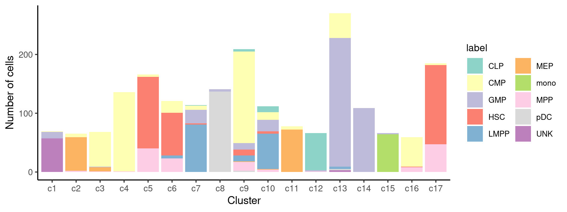
| Version | Author | Date |
|---|---|---|
| 6a9dead | kevinlkx | 2020-11-19 |
Percent stacked barplot for the counts of cell labels by clusters:
freq_cluster_celltype <- count(samples, vars=c("cluster_kmeans","label"))
n_colors <- length(levels(samples$label))
colors_labels <- brewer.pal(10, "Set3")

p.barplot.2 <- ggplot(freq_cluster_celltype, aes(fill=label, y=freq, x=cluster_kmeans)) +
  geom_bar(position="fill", stat="identity") +
  theme_classic() + xlab("Cluster") + ylab("Proportion of cells") +
  scale_fill_manual(values = colors_labels) +
  guides(fill=guide_legend(ncol=2)) +
  theme(
  legend.title = element_text(size = 10),
  legend.text = element_text(size = 8)
  )
print(p.barplot.2)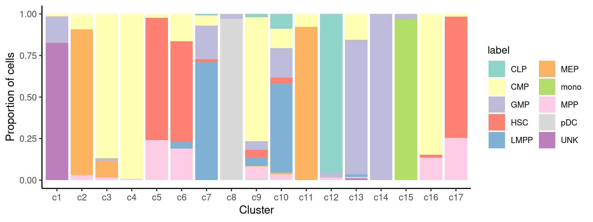
| Version | Author | Date |
|---|---|---|
| 6a9dead | kevinlkx | 2020-11-19 |
Binarized counts
Load the binarized data
data.dir <- "/project2/mstephens/kevinluo/scATACseq-topics/data/Buenrostro_2018/processed_data_Chen2019pipeline/"
load(file.path(data.dir, "Buenrostro_2018_binarized_counts.RData"))
cat(sprintf("%d x %d counts matrix.\n",nrow(counts),ncol(counts)))
rm(counts)
samples$cell <- rownames(samples)
samples$label <- as.factor(samples$label)
# 2034 x 101172 counts matrix.
Plot PCs of the topic proportions
We first use PCA to explore the structure inferred from the multinomial topic model with \(k = 11\):
out.dir <- "/project2/mstephens/kevinluo/scATACseq-topics/output/Buenrostro_2018_Chen2019pipeline/binarized/"
fit <- readRDS(file.path(out.dir, "/fit-Buenrostro2018-binarized-scd-ex-k=11.rds"))$fit

colors_topics <- c("#a6cee3","#1f78b4","#b2df8a","#33a02c","#fb9a99","#e31a1c",
                   "#fdbf6f","#ff7f00","#cab2d6","#6a3d9a","#ffff99")
Plot PCs of the topic proportions.
p.pca1.1 <- pca_plot(poisson2multinom(fit),pcs = 1:2,fill = "none")
p.pca1.2 <- pca_plot(poisson2multinom(fit),pcs = 3:4,fill = "none")
p.pca1.3 <- pca_plot(poisson2multinom(fit),pcs = 5:6,fill = "none")
p.pca1.4 <- pca_plot(poisson2multinom(fit),pcs = 7:8,fill = "none")
p.pca1.5 <- pca_plot(poisson2multinom(fit),pcs = 9:10,fill = "none")

plot_grid(p.pca1.1,p.pca1.2,p.pca1.3,p.pca1.4,p.pca1.5)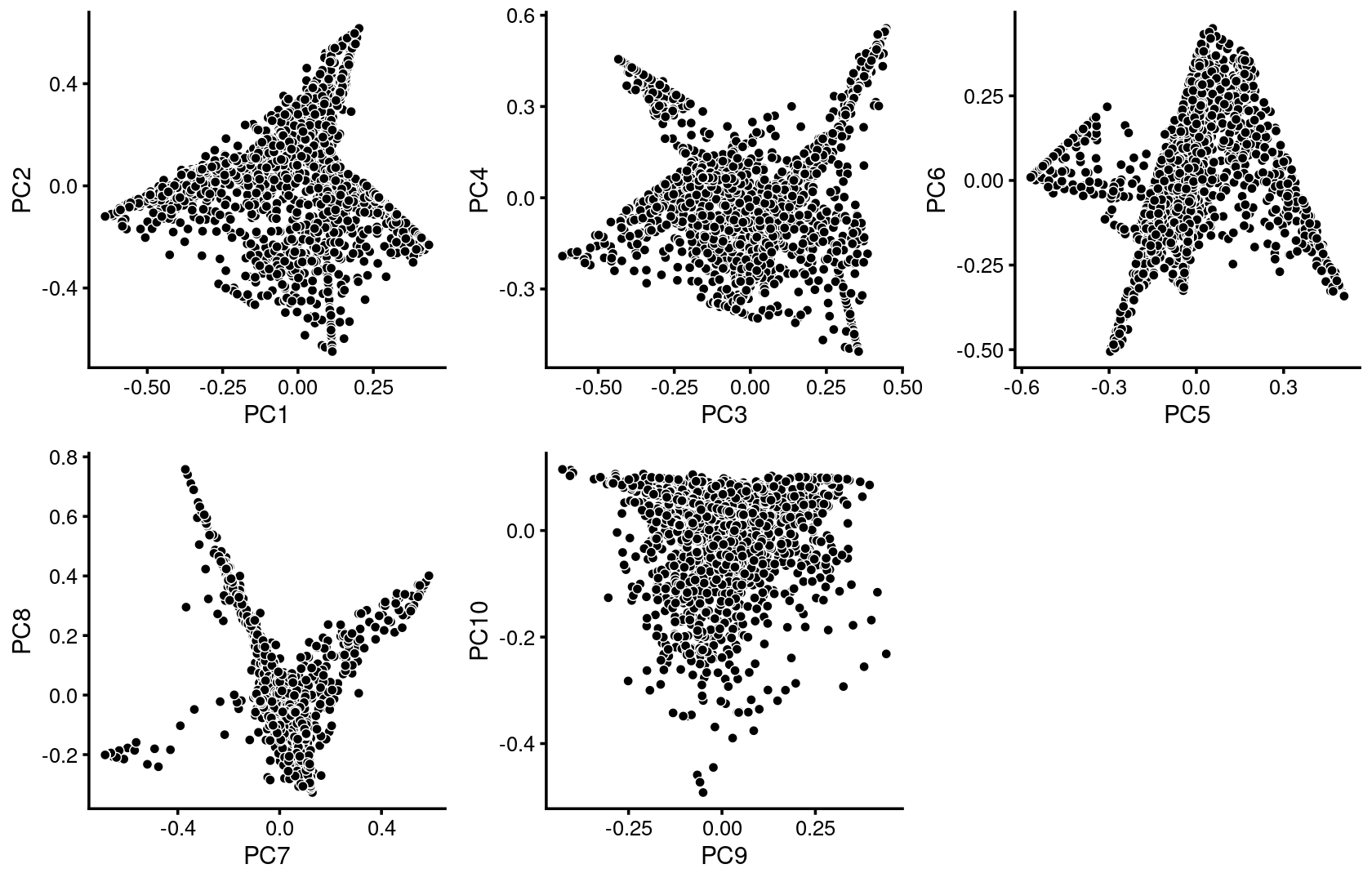
| Version | Author | Date |
|---|---|---|
| 6a9dead | kevinlkx | 2020-11-19 |
Some of the structure is more evident from “hexbin” plots showing the density of the points.
breaks <- c(0,1,5,10,100,Inf)
p.pca2.1 <- pca_hexbin_plot(poisson2multinom(fit), pcs = 1:2, breaks = breaks) + guides(fill = "none")
p.pca2.2 <- pca_hexbin_plot(poisson2multinom(fit), pcs = 3:4, breaks = breaks) + guides(fill = "none")
p.pca2.3 <- pca_hexbin_plot(poisson2multinom(fit), pcs = 5:6, breaks = breaks) + guides(fill = "none")
p.pca2.4 <- pca_hexbin_plot(poisson2multinom(fit), pcs = 7:8, breaks = breaks) + guides(fill = "none")
p.pca2.5 <- pca_hexbin_plot(poisson2multinom(fit), pcs = 9:10, breaks = breaks) + guides(fill = "none")

plot_grid(p.pca2.1,p.pca2.2,p.pca2.3,p.pca2.4,p.pca2.5)
| Version | Author | Date |
|---|---|---|
| 6a9dead | kevinlkx | 2020-11-19 |
Layer the cell labels onto the PC plots
Here, we layer the cell labels onto the PC plots.
p.pca3.1 <- labeled_pca_plot(fit,1:2,samples$label,font_size = 7,
                       legend_label = "Cell labels")
p.pca3.2 <- labeled_pca_plot(fit,3:4,samples$label,font_size = 7,
                       legend_label = "Cell labels")
p.pca3.3 <- labeled_pca_plot(fit,5:6,samples$label,font_size = 7,
                       legend_label = "Cell labels")
p.pca3.4 <- labeled_pca_plot(fit,7:8,samples$label,font_size = 7,
                       legend_label = "Cell labels")
p.pca3.5 <- labeled_pca_plot(fit,9:10,samples$label,font_size = 7,
                       legend_label = "Cell labels")

plot_grid(p.pca3.1,p.pca3.2,p.pca3.3,p.pca3.4,p.pca3.5)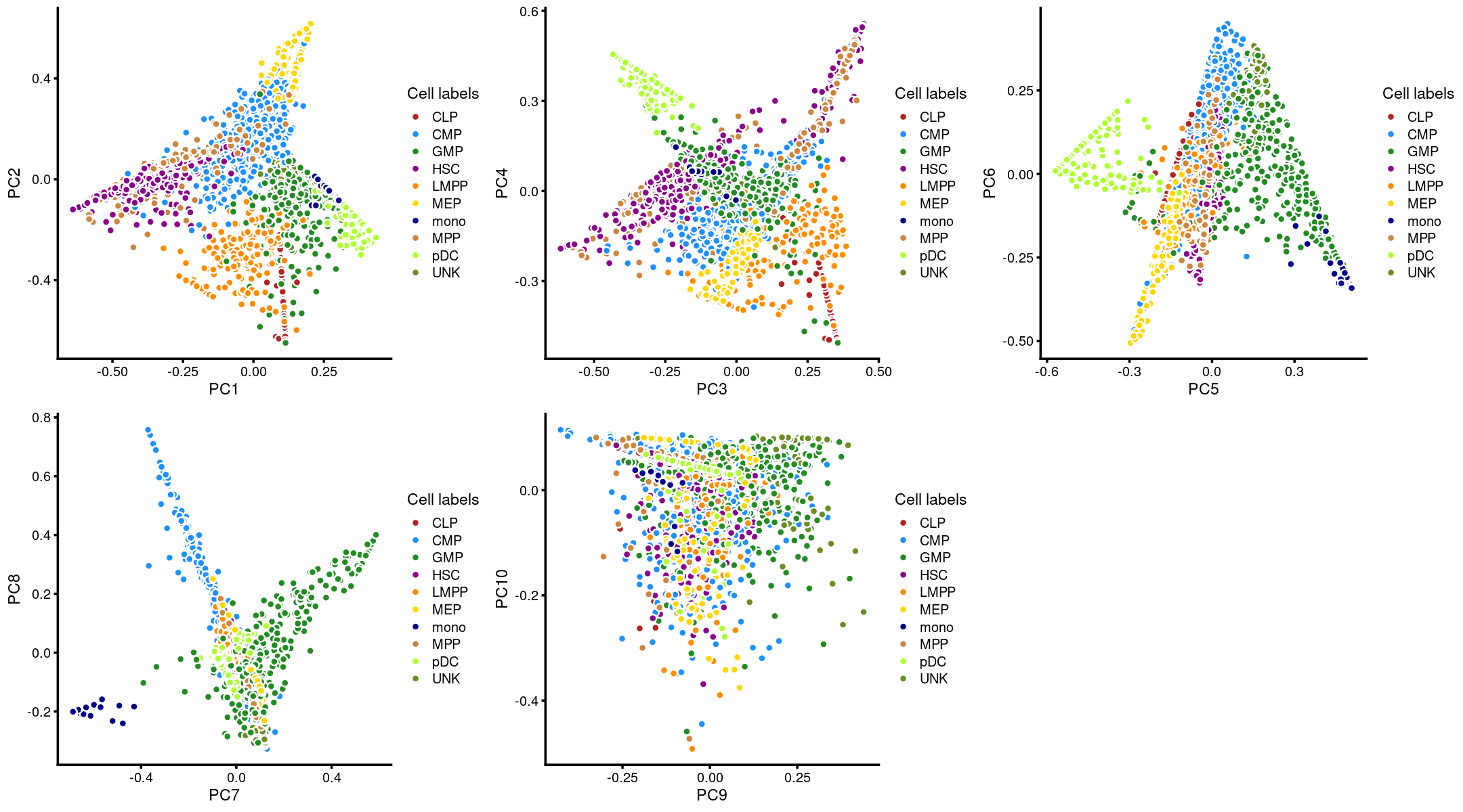
| Version | Author | Date |
|---|---|---|
| 6a9dead | kevinlkx | 2020-11-19 |
Visualize by structure plot grouped by cell labels.
set.seed(10)

samples$label <- as.factor(samples$label)

p.structure.1 <- structure_plot(poisson2multinom(fit),
                     grouping = samples[, "label"],
                     n = Inf,gap = 20,
                     perplexity = 50,topics = 1:11,colors = colors_topics,
                     num_threads = 4,verbose = FALSE)
# Perplexity automatically changed to 24 because original setting of 50 was too large for the number of samples (78)
# Perplexity automatically changed to 44 because original setting of 50 was too large for the number of samples (138)
# Perplexity automatically changed to 20 because original setting of 50 was too large for the number of samples (64)
# Perplexity automatically changed to 46 because original setting of 50 was too large for the number of samples (142)
# Perplexity automatically changed to 45 because original setting of 50 was too large for the number of samples (141)
# Perplexity automatically changed to 18 because original setting of 50 was too large for the number of samples (60)

print(p.structure.1)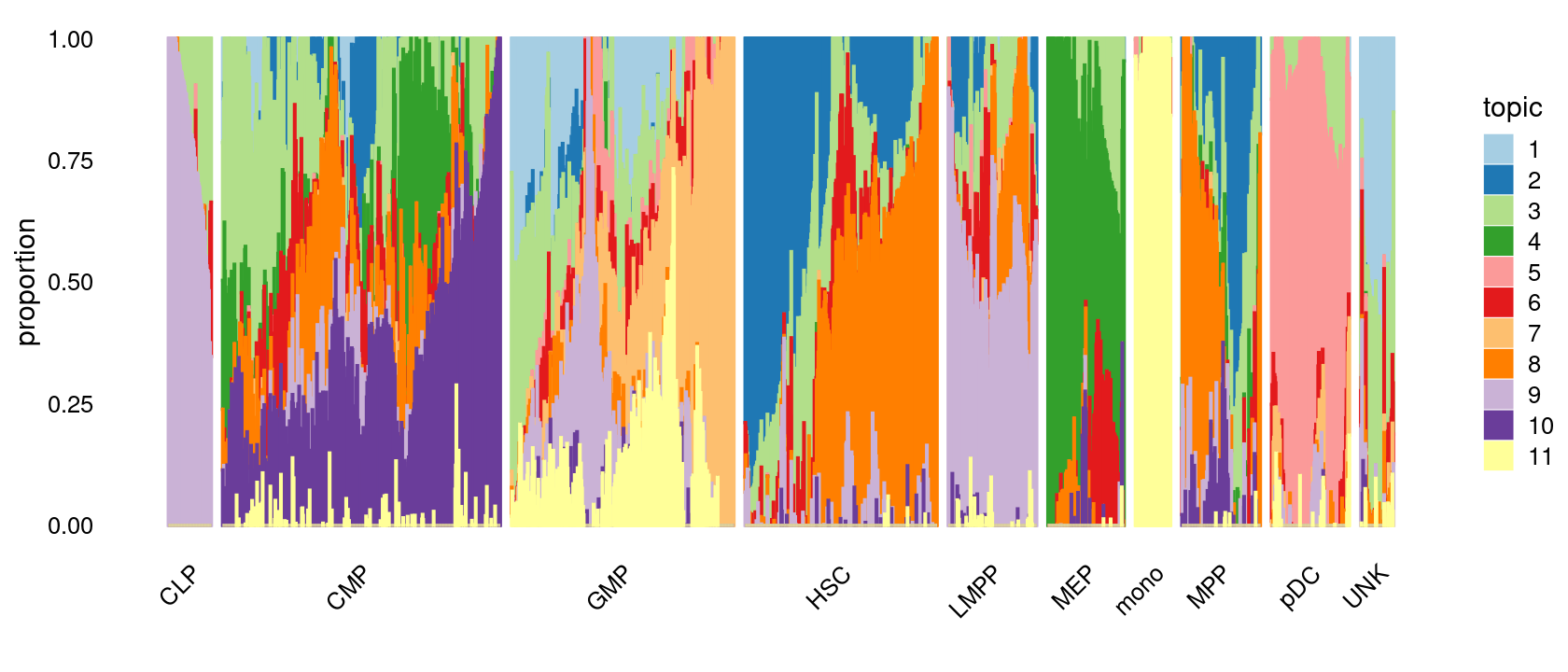
| Version | Author | Date |
|---|---|---|
| 6a9dead | kevinlkx | 2020-11-19 |
k-means clustering on topic proportions
Define clusters using k-means, and then create structure plot based on the clusters from k-means.
Define clusters using k-means with \(k = 10\):
set.seed(10)

clusters.10 <- factor(kmeans(poisson2multinom(fit)$L,centers = 10)$cluster)
print(sort(table(clusters.10),decreasing = TRUE))
# clusters.10
#   9   1   6   7   4  10   2   8   5   3
# 332 308 304 254 179 170 157 132 108  90
Structure plot based on k-means clusters
p.structure.2 <- structure_plot(poisson2multinom(fit),
                     grouping = clusters.10,
                     # rows = order(samples$label), # samples are grouped by clusters first, then by celltype labels
                     n = Inf,gap = 20,
                     perplexity = 50,topics = 1:11,colors = colors_topics,
                     num_threads = 4,verbose = FALSE)
# Perplexity automatically changed to 28 because original setting of 50 was too large for the number of samples (90)
# Perplexity automatically changed to 34 because original setting of 50 was too large for the number of samples (108)
# Perplexity automatically changed to 42 because original setting of 50 was too large for the number of samples (132)
print(p.structure.2)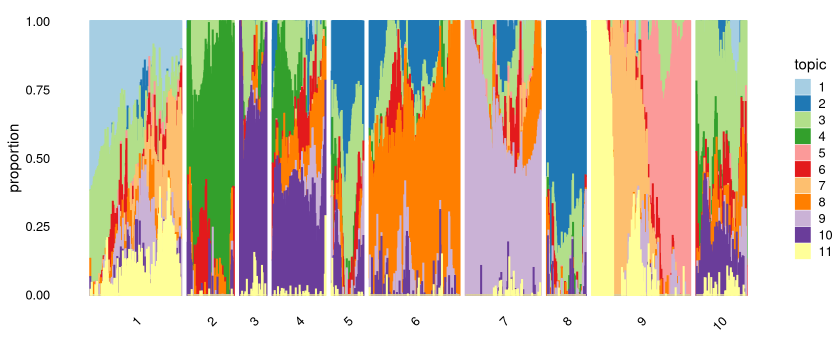
| Version | Author | Date |
|---|---|---|
| 6a9dead | kevinlkx | 2020-11-19 |
Define clusters using k-means with \(k = 15\):
set.seed(10)

clusters.15 <- factor(kmeans(poisson2multinom(fit)$L,centers = 15)$cluster)
print(sort(table(clusters.15),decreasing = TRUE))
# clusters.15
#   1   5   7   4   9  11   8   2  15  13   6  10   3  12  14
# 279 213 199 175 144 132 131 122 119  99  97  93  89  71  71
Structure plot based on k-means clusters
p.structure.3 <- structure_plot(poisson2multinom(fit),
                     grouping = clusters.15,
                     # rows = order(samples$label), # samples are grouped by clusters first, then by celltype labels
                     n = Inf,gap = 20,
                     perplexity = 50,topics = 1:11, colors = colors_topics,
                     num_threads = 4,verbose = FALSE)
# Perplexity automatically changed to 39 because original setting of 50 was too large for the number of samples (122)
# Perplexity automatically changed to 28 because original setting of 50 was too large for the number of samples (89)
# Perplexity automatically changed to 31 because original setting of 50 was too large for the number of samples (97)
# Perplexity automatically changed to 42 because original setting of 50 was too large for the number of samples (131)
# Perplexity automatically changed to 46 because original setting of 50 was too large for the number of samples (144)
# Perplexity automatically changed to 29 because original setting of 50 was too large for the number of samples (93)
# Perplexity automatically changed to 42 because original setting of 50 was too large for the number of samples (132)
# Perplexity automatically changed to 22 because original setting of 50 was too large for the number of samples (71)
# Perplexity automatically changed to 31 because original setting of 50 was too large for the number of samples (99)
# Perplexity automatically changed to 22 because original setting of 50 was too large for the number of samples (71)
# Perplexity automatically changed to 38 because original setting of 50 was too large for the number of samples (119)
print(p.structure.3)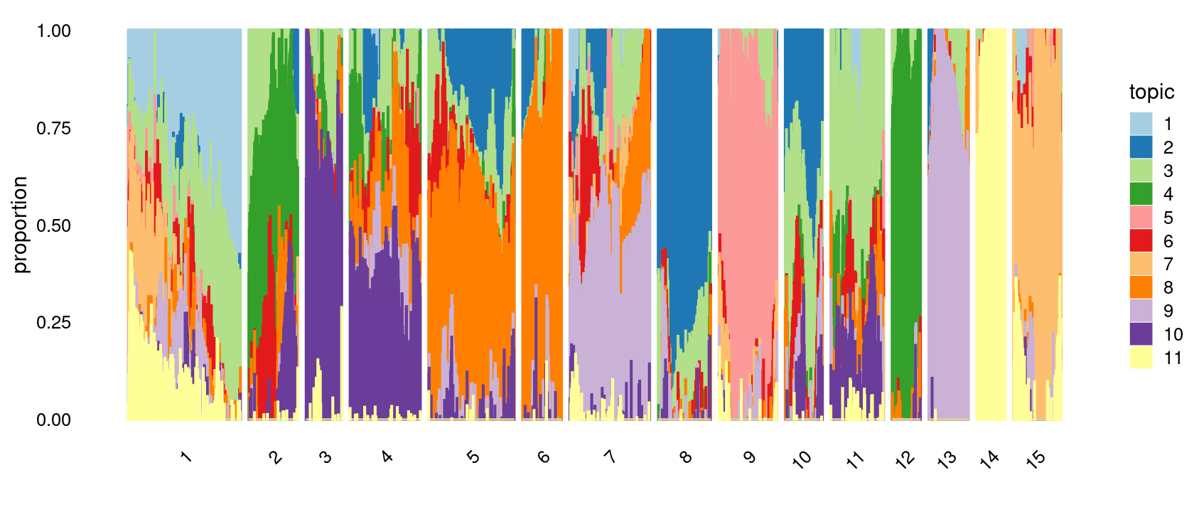
| Version | Author | Date |
|---|---|---|
| 6a9dead | kevinlkx | 2020-11-19 |
Define clusters using k-means with \(k = 20\):
set.seed(10)

clusters.20 <- factor(kmeans(poisson2multinom(fit)$L,centers = 20)$cluster)
print(sort(table(clusters.20),decreasing = TRUE))
# clusters.20
#  19   7   1   9   4  14   2  11   6  13   8   3  20  16  12  17  15   5  10  18
# 212 187 177 143 128 117 107 102  97  93  85  77  76  75  70  66  60  58  53  51
Structure plot based on k-means clusters
p.structure.4 <- structure_plot(poisson2multinom(fit),
                     grouping = clusters.20,
                     # rows = order(samples$label), # samples are grouped by clusters first, then by celltype labels
                     n = Inf,gap = 20,
                     perplexity = 50,topics = 1:11, colors = colors_topics,
                     num_threads = 4,verbose = FALSE)
# Perplexity automatically changed to 34 because original setting of 50 was too large for the number of samples (107)
# Perplexity automatically changed to 24 because original setting of 50 was too large for the number of samples (77)
# Perplexity automatically changed to 41 because original setting of 50 was too large for the number of samples (128)
# Perplexity automatically changed to 18 because original setting of 50 was too large for the number of samples (58)
# Perplexity automatically changed to 31 because original setting of 50 was too large for the number of samples (97)
# Perplexity automatically changed to 27 because original setting of 50 was too large for the number of samples (85)
# Perplexity automatically changed to 46 because original setting of 50 was too large for the number of samples (143)
# Perplexity automatically changed to 16 because original setting of 50 was too large for the number of samples (53)
# Perplexity automatically changed to 32 because original setting of 50 was too large for the number of samples (102)
# Perplexity automatically changed to 22 because original setting of 50 was too large for the number of samples (70)
# Perplexity automatically changed to 29 because original setting of 50 was too large for the number of samples (93)
# Perplexity automatically changed to 37 because original setting of 50 was too large for the number of samples (117)
# Perplexity automatically changed to 18 because original setting of 50 was too large for the number of samples (60)
# Perplexity automatically changed to 23 because original setting of 50 was too large for the number of samples (75)
# Perplexity automatically changed to 20 because original setting of 50 was too large for the number of samples (66)
# Perplexity automatically changed to 15 because original setting of 50 was too large for the number of samples (51)
# Perplexity automatically changed to 24 because original setting of 50 was too large for the number of samples (76)
print(p.structure.4)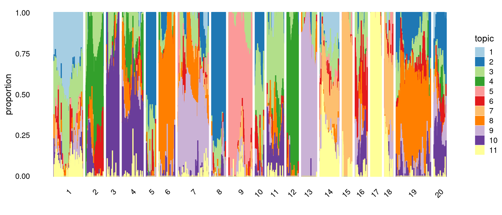
| Version | Author | Date |
|---|---|---|
| 6a9dead | kevinlkx | 2020-11-19 |
Refine clusters
We then further refine the clusters based on k-means result with \(k = 20\): merge clusters 3, 4; merge clusters 5 and 8; merge clusters 6 and 19; merge clusters 14 and 18; merge clusters 16 and 20
clusters.merged <- clusters.20
clusters.merged[clusters.20 %in% c(3,4)] <- 3
clusters.merged[clusters.20 %in% c(5,8)] <- 5
clusters.merged[clusters.20 %in% c(6,19)] <- 6
clusters.merged[clusters.20 %in% c(14,18)] <- 14
clusters.merged[clusters.20 %in% c(16,20)] <- 16

clusters.merged <- factor(clusters.merged, labels = paste0("c", c(1:length(unique(clusters.merged)))))
samples$cluster_kmeans <- clusters.merged
table(clusters.merged)
# clusters.merged
#  c1  c2  c3  c4  c5  c6  c7  c8  c9 c10 c11 c12 c13 c14 c15
# 177 107 205 143 309 187 143  53 102  70  93 168  60 151  66
p.structure.refined <- structure_plot(poisson2multinom(fit),
grouping = clusters.merged,
# rows = order(samples$label), # samples are grouped by clusters first, then by celltype labels
n = Inf,gap = 20,
perplexity = 50,topics = 1:11,colors = colors_topics,
num_threads = 4,verbose = FALSE)
# Perplexity automatically changed to 34 because original setting of 50 was too large for the number of samples (107)
# Perplexity automatically changed to 46 because original setting of 50 was too large for the number of samples (143)
# Perplexity automatically changed to 46 because original setting of 50 was too large for the number of samples (143)
# Perplexity automatically changed to 16 because original setting of 50 was too large for the number of samples (53)
# Perplexity automatically changed to 32 because original setting of 50 was too large for the number of samples (102)
# Perplexity automatically changed to 22 because original setting of 50 was too large for the number of samples (70)
# Perplexity automatically changed to 29 because original setting of 50 was too large for the number of samples (93)
# Perplexity automatically changed to 18 because original setting of 50 was too large for the number of samples (60)
# Perplexity automatically changed to 49 because original setting of 50 was too large for the number of samples (151)
# Perplexity automatically changed to 20 because original setting of 50 was too large for the number of samples (66)
print(p.structure.refined)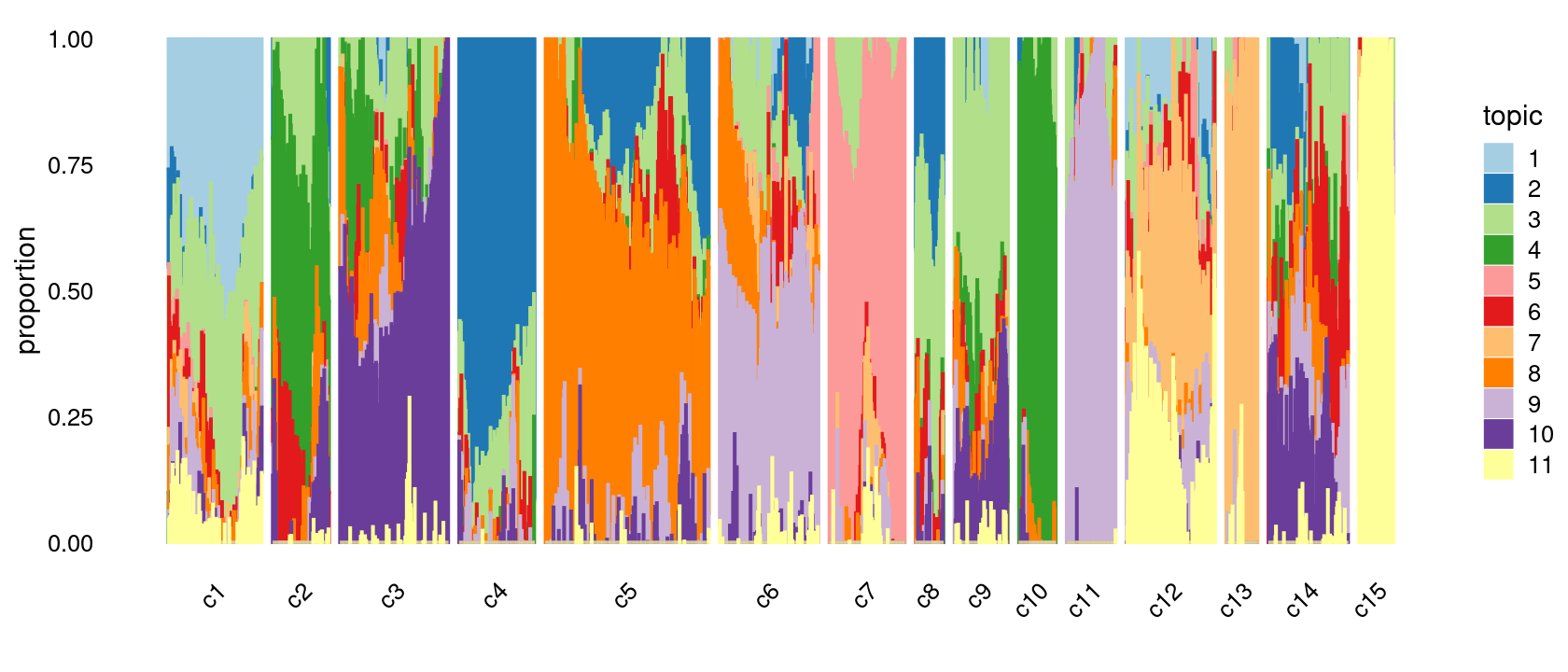
| Version | Author | Date |
|---|---|---|
| 6a9dead | kevinlkx | 2020-11-19 |
Group samples by k-means clusters first, then by celltype labels:
p.structure.refined <- structure_plot(poisson2multinom(fit),
                     grouping = clusters.merged,
                     rows = order(samples$label), # samples are grouped by clusters first, then by celltype labels
                     n = Inf,gap = 20,
                     perplexity = 50,topics = 1:11,colors = colors_topics,
                     num_threads = 4,verbose = FALSE)
print(p.structure.refined)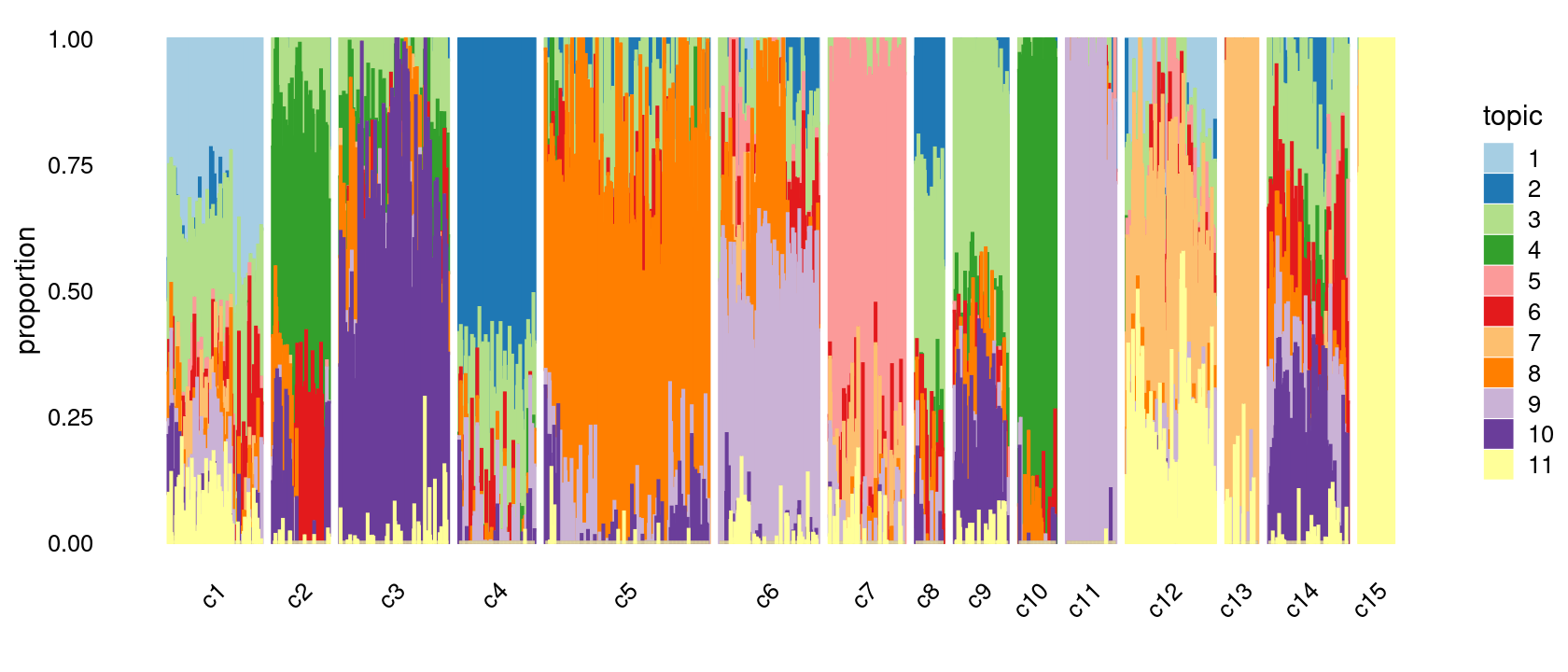
| Version | Author | Date |
|---|---|---|
| 6a9dead | kevinlkx | 2020-11-19 |
The clusters defined by k-means on topic proportions reasonably identify the clusters shown in the PCA hexbin plots (below).
p.pca.4.1 <- labeled_pca_plot(fit,1:2,samples$cluster_kmeans,font_size = 7,
                       legend_label = "cluster_kmeans")
p.pca.4.2 <- labeled_pca_plot(fit,3:4,samples$cluster_kmeans,font_size = 7,
                       legend_label = "cluster_kmeans")
p.pca.4.3 <- labeled_pca_plot(fit,5:6,samples$cluster_kmeans,font_size = 7,
                       legend_label = "cluster_kmeans")
p.pca.4.4 <- labeled_pca_plot(fit,7:8,samples$cluster_kmeans,font_size = 7,
                       legend_label = "cluster_kmeans")
p.pca.4.5 <- labeled_pca_plot(fit,9:10,samples$cluster_kmeans,font_size = 7,
                       legend_label = "cluster_kmeans")
plot_grid(p.pca.4.1,p.pca.4.2,p.pca.4.3,p.pca.4.4,p.pca.4.5)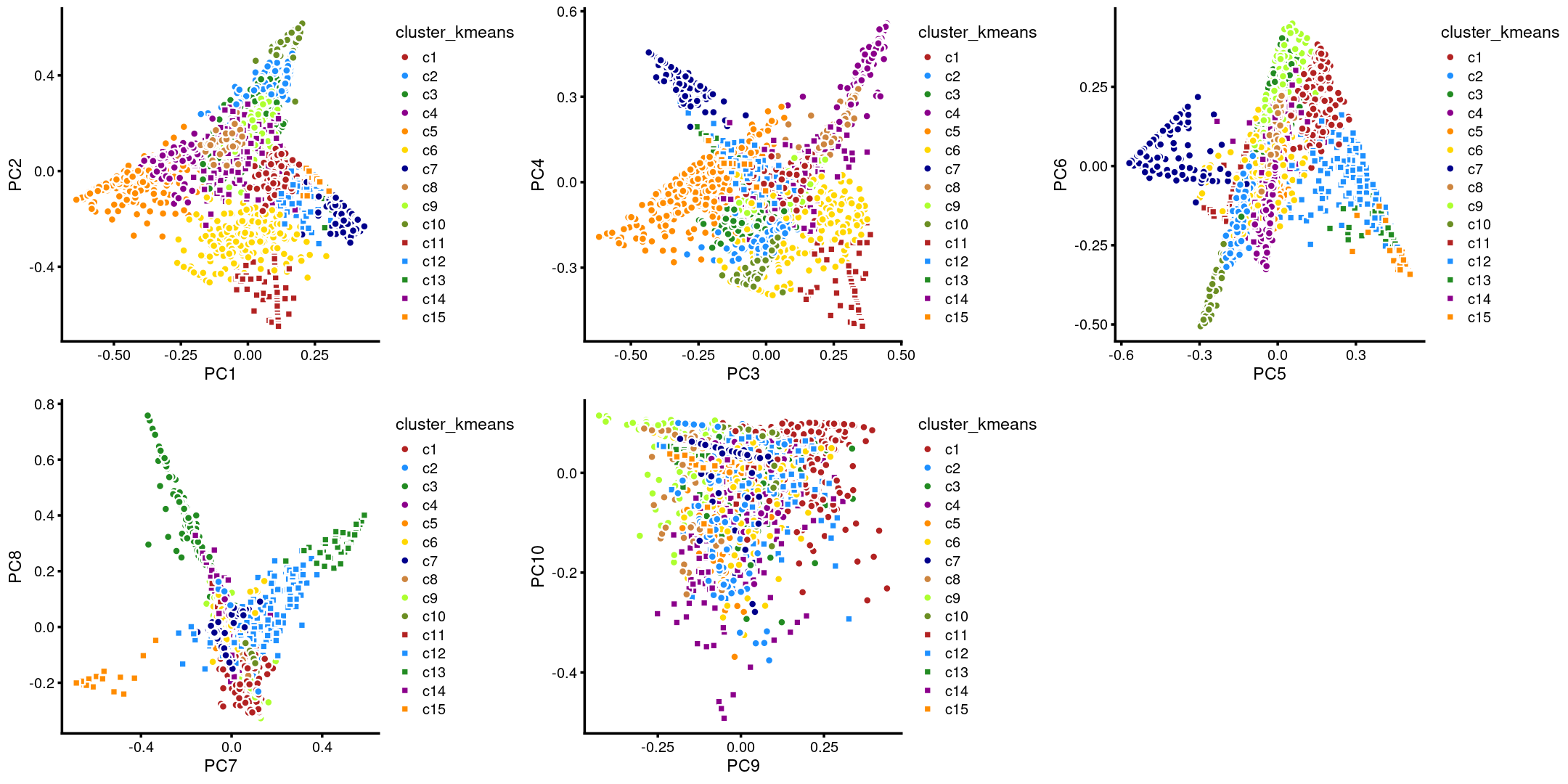
| Version | Author | Date |
|---|---|---|
| 6a9dead | kevinlkx | 2020-11-19 |
plot_grid(p.pca2.1,p.pca2.2,p.pca2.3,p.pca2.4,p.pca2.5)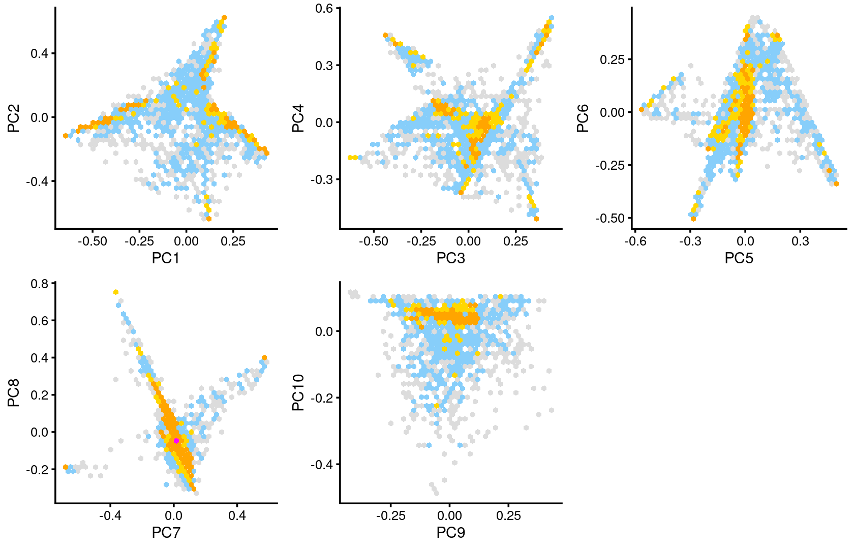
| Version | Author | Date |
|---|---|---|
| 6a9dead | kevinlkx | 2020-11-19 |
We then label the cells in each cluster with the known cell labels.
Cell labels:
samples$label <- as.factor(samples$label)
cat(length(levels(samples$label)), "cell labels. \n")
table(samples$label)
# 10 cell labels.
#
#  CLP  CMP  GMP  HSC LMPP  MEP mono  MPP  pDC  UNK
#   78  502  402  347  160  138   64  142  141   60
We can see a few clusters are dominated by one major cell type:
freq_cluster_cells <- with(samples,table(label,cluster_kmeans))
print(freq_cluster_cells)
#       cluster_kmeans
# label   c1  c2  c3  c4  c5  c6  c7  c8  c9 c10 c11 c12 c13 c14 c15
#   CLP    0   0   0   0   0  12   0   0   1   0  63   0   0   2   0
#   CMP   16  33 202   3  25   7   0  12  89   5   0   1   0 109   0
#   GMP  102   1   0   0   0  41   3   0   3   0  10 165  60  15   2
#   HSC    0   0   0 109 210   0   0  22   1   0   0   0   0   5   0
#   LMPP   1   0   0   0   1 125   0   0   1   0  20   2   0  10   0
#   MEP    0  70   2   0   0   0   0   0   1  65   0   0   0   0   0
#   mono   0   0   0   0   0   0   0   0   0   0   0   0   0   0  64
#   MPP    0   3   1  31  73   1   0  19   5   0   0   0   0   9   0
#   pDC    0   0   0   0   0   0 140   0   0   0   0   0   0   1   0
#   UNK   58   0   0   0   0   1   0   0   1   0   0   0   0   0   0
Plot the distribution of cell labels by clusters.
Stacked barplot for the counts of cell labels by clusters:
library(plyr);library(dplyr)
library(RColorBrewer)

freq_cluster_celltype <- count(samples, vars=c("cluster_kmeans","label"))
n_colors <- length(levels(samples$label))
colors_labels <- brewer.pal(10, "Set3")

# stacked barplot for the counts of cell labels by clusters
p.barplot.1 <- ggplot(freq_cluster_celltype, aes(fill=label, y=freq, x=cluster_kmeans)) +
  geom_bar(position="stack", stat="identity") +
  theme_classic() + xlab("Cluster") + ylab("Number of cells") +
  scale_fill_manual(values = colors_labels) +
  guides(fill=guide_legend(ncol=2)) +
  theme(
  legend.title = element_text(size = 10),
  legend.text = element_text(size = 8)
  )
print(p.barplot.1)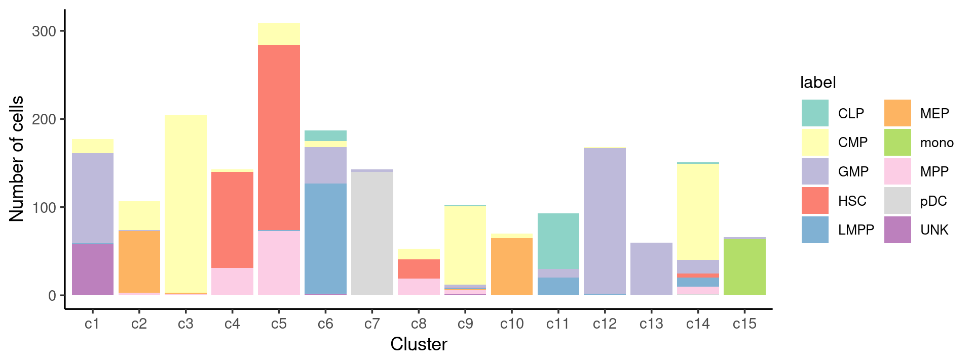
| Version | Author | Date |
|---|---|---|
| 6a9dead | kevinlkx | 2020-11-19 |
Percent stacked barplot for the counts of cell labels by clusters:
freq_cluster_celltype <- count(samples, vars=c("cluster_kmeans","label"))
n_colors <- length(levels(samples$label))
colors_labels <- brewer.pal(10, "Set3")

p.barplot.2 <- ggplot(freq_cluster_celltype, aes(fill=label, y=freq, x=cluster_kmeans)) +
  geom_bar(position="fill", stat="identity") +
  theme_classic() + xlab("Cluster") + ylab("Proportion of cells") +
  scale_fill_manual(values = colors_labels) +
  guides(fill=guide_legend(ncol=2)) +
  theme(
  legend.title = element_text(size = 10),
  legend.text = element_text(size = 8)
  )
print(p.barplot.2)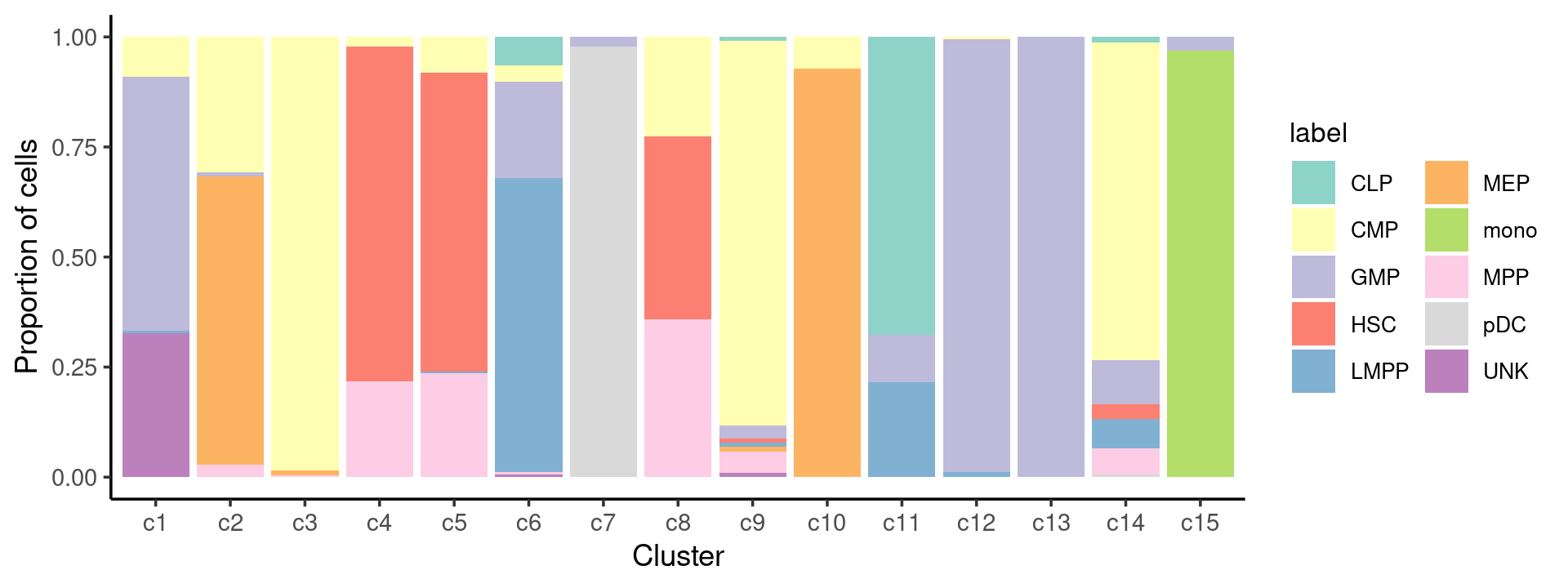
| Version | Author | Date |
|---|---|---|
| 6a9dead | kevinlkx | 2020-11-19 |
sessionInfo()
# R version 3.6.1 (2019-07-05)
# Platform: x86_64-pc-linux-gnu (64-bit)
# Running under: Scientific Linux 7.4 (Nitrogen)
#
# Matrix products: default
# BLAS/LAPACK: /software/openblas-0.2.19-el7-x86_64/lib/libopenblas_haswellp-r0.2.19.so
#
# locale:
#  [1] LC_CTYPE=en_US.UTF-8       LC_NUMERIC=C
#  [3] LC_TIME=en_US.UTF-8        LC_COLLATE=en_US.UTF-8
#  [5] LC_MONETARY=en_US.UTF-8    LC_MESSAGES=en_US.UTF-8
#  [7] LC_PAPER=en_US.UTF-8       LC_NAME=C
#  [9] LC_ADDRESS=C               LC_TELEPHONE=C
# [11] LC_MEASUREMENT=en_US.UTF-8 LC_IDENTIFICATION=C
#
# attached base packages:
# [1] stats     graphics  grDevices utils     datasets  methods   base
#
# other attached packages:
# [1] RColorBrewer_1.1-2 plyr_1.8.6         fastTopics_0.3-180 cowplot_1.1.0
# [5] ggplot2_3.3.2      dplyr_1.0.2        Matrix_1.2-18      workflowr_1.6.2
#
# loaded via a namespace (and not attached):
#  [1] ggrepel_0.8.2      Rcpp_1.0.5         lattice_0.20-41    tidyr_1.1.2
#  [5] prettyunits_1.1.1  rprojroot_1.3-2    digest_0.6.27      R6_2.5.0
#  [9] backports_1.2.0    MatrixModels_0.4-1 evaluate_0.14      coda_0.19-3
# [13] httr_1.4.2         pillar_1.4.7       rlang_0.4.8        progress_1.2.2
# [17] lazyeval_0.2.2     data.table_1.13.2  irlba_2.3.3        SparseM_1.77
# [21] whisker_0.4        hexbin_1.28.1      rmarkdown_2.5      labeling_0.4.2
# [25] Rtsne_0.15         stringr_1.4.0      htmlwidgets_1.5.2  munsell_0.5.0
# [29] compiler_3.6.1     httpuv_1.5.4       xfun_0.19          pkgconfig_2.0.3
# [33] mcmc_0.9-7         htmltools_0.5.0    tidyselect_1.1.0   tibble_3.0.4
# [37] quadprog_1.5-7     viridisLite_0.3.0  crayon_1.3.4       withr_2.3.0
# [41] later_1.1.0.1      MASS_7.3-53        grid_3.6.1         jsonlite_1.6
# [45] gtable_0.3.0       lifecycle_0.2.0    git2r_0.27.1       magrittr_1.5
# [49] scales_1.1.1       RcppParallel_5.0.2 stringi_1.5.3      farver_2.0.3
# [53] fs_1.3.1           promises_1.1.1     ellipsis_0.3.1     generics_0.0.2
# [57] vctrs_0.3.5        tools_3.6.1        glue_1.4.2         purrr_0.3.4
# [61] hms_0.5.3          yaml_2.2.0         colorspace_2.0-0   plotly_4.9.0
# [65] knitr_1.30         quantreg_5.41      MCMCpack_1.4-4