Compare PC plots of topic proportions from fastTopic with different K in Buenrostro et al (2018) scATAC-seq data
Kaixuan Luo
Last updated: 2020-11-06
Checks: 7 0
Knit directory: scATACseq-topics/
This reproducible R Markdown analysis was created with workflowr (version 1.6.2). The Checks tab describes the reproducibility checks that were applied when the results were created. The Past versions tab lists the development history.
Great! Since the R Markdown file has been committed to the Git repository, you know the exact version of the code that produced these results.
Great job! The global environment was empty. Objects defined in the global environment can affect the analysis in your R Markdown file in unknown ways. For reproduciblity it’s best to always run the code in an empty environment.
The command set.seed(20200729) was run prior to running the code in the R Markdown file. Setting a seed ensures that any results that rely on randomness, e.g. subsampling or permutations, are reproducible.
Great job! Recording the operating system, R version, and package versions is critical for reproducibility.
Nice! There were no cached chunks for this analysis, so you can be confident that you successfully produced the results during this run.
Great job! Using relative paths to the files within your workflowr project makes it easier to run your code on other machines.
Great! You are using Git for version control. Tracking code development and connecting the code version to the results is critical for reproducibility.
The results in this page were generated with repository version 1826fa0. See the Past versions tab to see a history of the changes made to the R Markdown and HTML files.
Note that you need to be careful to ensure that all relevant files for the analysis have been committed to Git prior to generating the results (you can use wflow_publish or wflow_git_commit). workflowr only checks the R Markdown file, but you know if there are other scripts or data files that it depends on. Below is the status of the Git repository when the results were generated:
Ignored files:
    Ignored:    .Rhistory
    Ignored:    .Rproj.user/

Untracked files:
    Untracked:  analysis/clusters_pca_structure_Cusanovich2018.Rmd

Unstaged changes:
    Modified:   analysis/index.Rmd
    Modified:   analysis/plots_Lareau2019_bonemarrow.Rmd
    Modified:   scripts/fit_all_models_Lareau2019.sh
Note that any generated files, e.g. HTML, png, CSS, etc., are not included in this status report because it is ok for generated content to have uncommitted changes.
These are the previous versions of the repository in which changes were made to the R Markdown (analysis/compare_pca_clusters_Buenrostro_2018.Rmd) and HTML (docs/compare_pca_clusters_Buenrostro_2018.html) files. If you’ve configured a remote Git repository (see ?wflow_git_remote), click on the hyperlinks in the table below to view the files as they were in that past version.
| File | Version | Author | Date | Message |
|---|---|---|---|---|
| Rmd | 1826fa0 | kevinlkx | 2020-11-06 | add binarized data |
| html | fb6a121 | kevinlkx | 2020-11-06 | Build site. |
| Rmd | fbe50bc | kevinlkx | 2020-11-06 | add binarized data |
| html | 33925f4 | kevinlkx | 2020-11-05 | Build site. |
| Rmd | aa4715c | kevinlkx | 2020-11-05 | PCA plots for unbinarized data |
Here we explore the structure in the Buenrostro et al (2018) scATAC-seq data inferred from the multinomial topic model with different numbers of \(k\).
Load packages and some functions used in this analysis.
library(Matrix)
library(ggplot2)
library(cowplot)
library(fastTopics)
source("code/plots.R")
We applied the analysis both unbinarized counts and binarized scATAC-seq data.
Unbinarized counts
Load the data
data.dir <- "/project2/mstephens/kevinluo/scATACseq-topics/data/Buenrostro_2018/processed_data/"
load(file.path(data.dir, "Buenrostro_2018_counts.RData"))
cat(sprintf("%d x %d counts matrix.\n",nrow(counts),ncol(counts)))
rm(counts)
samples$label <- as.factor(samples$label)
# 2034 x 101172 counts matrix.
Plot PCs of the topic proportions
We first use PCA to explore the structure inferred from the multinomial topic model with different numbers of \(k\):
k = 10
Load the \(k = 10\) Poisson NMF fit.
out.dir <- "/project2/mstephens/kevinluo/scATACseq-topics/output/Buenrostro_2018/unbinarized/"
fit <- readRDS(file.path(out.dir, "/fit-Buenrostro2018-scd-ex-k=10.rds"))$fit
Plot PCs of the topic proportions.
p.pca1.1 <- pca_plot(poisson2multinom(fit),pcs = 1:2,fill = "none")
p.pca1.2 <- pca_plot(poisson2multinom(fit),pcs = 3:4,fill = "none")
p.pca1.3 <- pca_plot(poisson2multinom(fit),pcs = 5:6,fill = "none")
p.pca1.4 <- pca_plot(poisson2multinom(fit),pcs = 7:8,fill = "none")

plot_grid(p.pca1.1,p.pca1.2,p.pca1.3,p.pca1.4)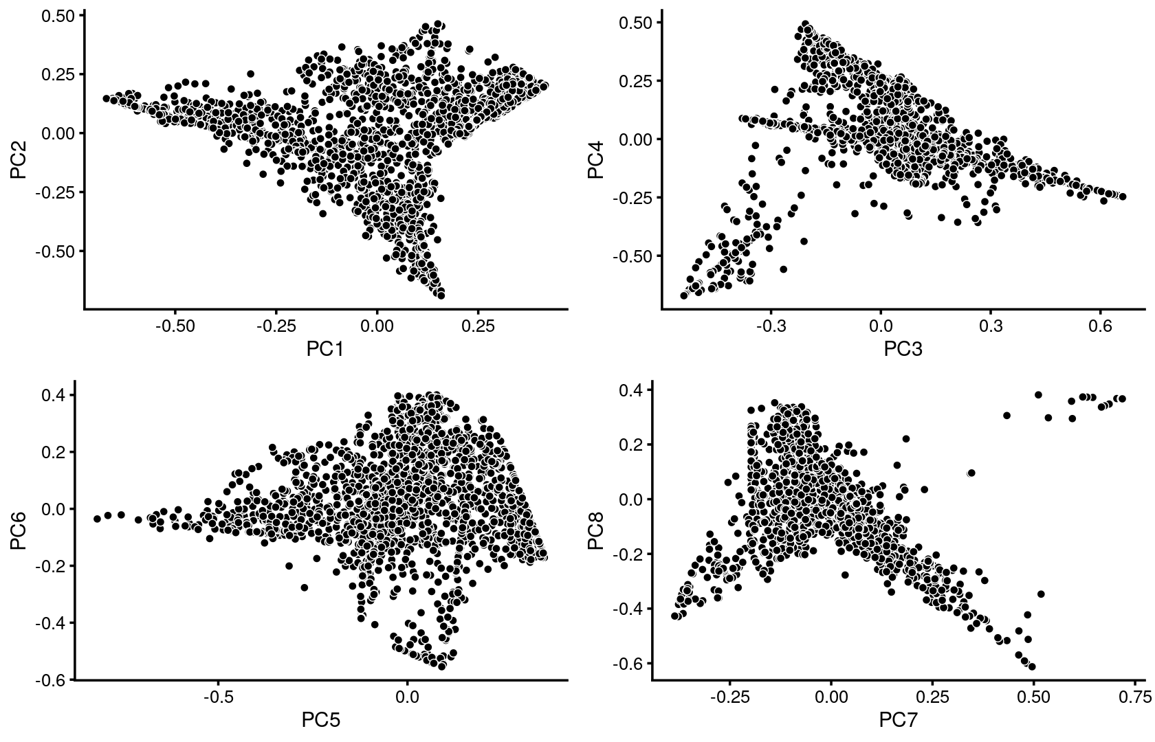
| Version | Author | Date |
|---|---|---|
| fb6a121 | kevinlkx | 2020-11-06 |
Some of the structure is more evident from “hexbin” plots showing the density of the points.
breaks <- c(0,1,5,10,100,Inf)
p.pca2.1 <- pca_hexbin_plot(poisson2multinom(fit), pcs = 1:2, breaks = breaks) + guides(fill = "none")
p.pca2.2 <- pca_hexbin_plot(poisson2multinom(fit), pcs = 3:4, breaks = breaks) + guides(fill = "none")
p.pca2.3 <- pca_hexbin_plot(poisson2multinom(fit), pcs = 5:6, breaks = breaks) + guides(fill = "none")
p.pca2.4 <- pca_hexbin_plot(poisson2multinom(fit), pcs = 7:8, breaks = breaks) + guides(fill = "none")

plot_grid(p.pca2.1,p.pca2.2,p.pca2.3,p.pca2.4)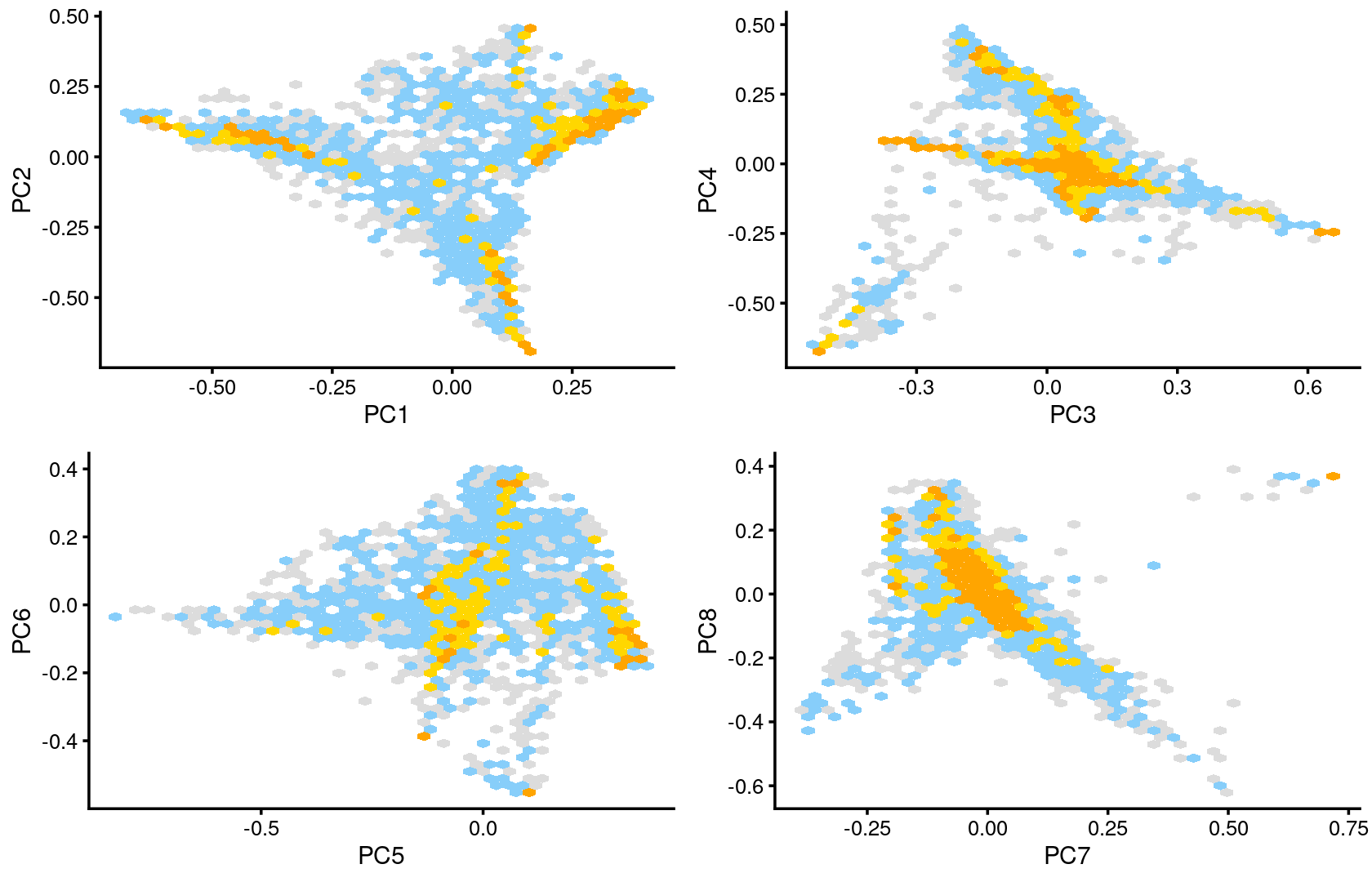
| Version | Author | Date |
|---|---|---|
| fb6a121 | kevinlkx | 2020-11-06 |
Next, we layer the cell labels onto the PC plots.
p.pca3.1 <- labeled_pca_plot(fit,1:2,samples$label,font_size = 7,
                       legend_label = "Cell labels")
p.pca3.2 <- labeled_pca_plot(fit,3:4,samples$label,font_size = 7,
                       legend_label = "Cell labels")
p.pca3.3 <- labeled_pca_plot(fit,5:6,samples$label,font_size = 7,
                       legend_label = "Cell labels")
p.pca3.4 <- labeled_pca_plot(fit,7:8,samples$label,font_size = 7,
                       legend_label = "Cell labels")

plot_grid(p.pca3.1,p.pca3.2,p.pca3.3,p.pca3.4)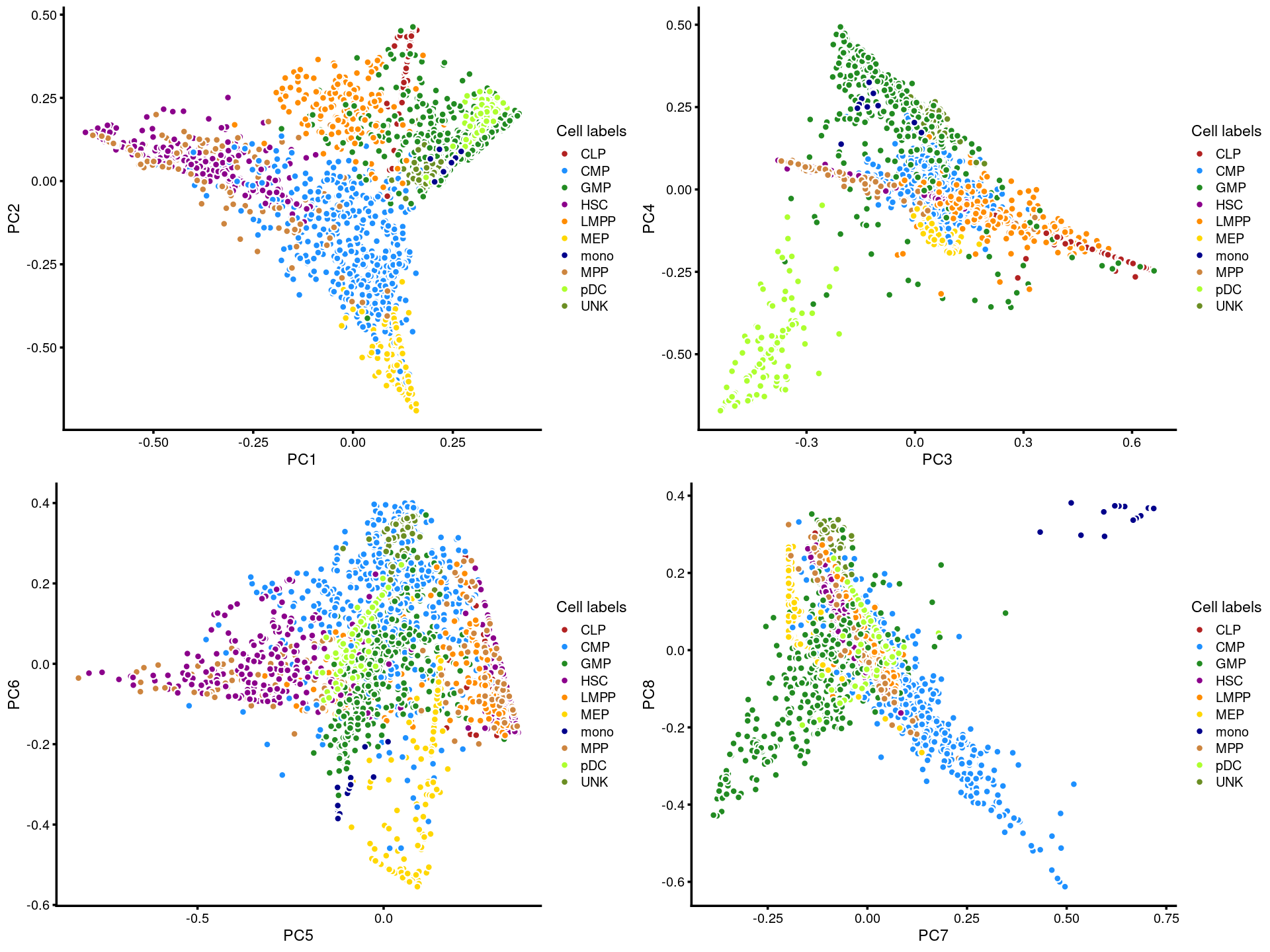
| Version | Author | Date |
|---|---|---|
| fb6a121 | kevinlkx | 2020-11-06 |
k = 11
Load the \(k = 11\) Poisson NMF fit.
out.dir <- "/project2/mstephens/kevinluo/scATACseq-topics/output/Buenrostro_2018/unbinarized/"
fit <- readRDS(file.path(out.dir, "/fit-Buenrostro2018-scd-ex-k=11.rds"))$fit
Plot PCs of the topic proportions.
p.pca1.1 <- pca_plot(poisson2multinom(fit),pcs = 1:2,fill = "none")
p.pca1.2 <- pca_plot(poisson2multinom(fit),pcs = 3:4,fill = "none")
p.pca1.3 <- pca_plot(poisson2multinom(fit),pcs = 5:6,fill = "none")
p.pca1.4 <- pca_plot(poisson2multinom(fit),pcs = 7:8,fill = "none")

plot_grid(p.pca1.1,p.pca1.2,p.pca1.3,p.pca1.4)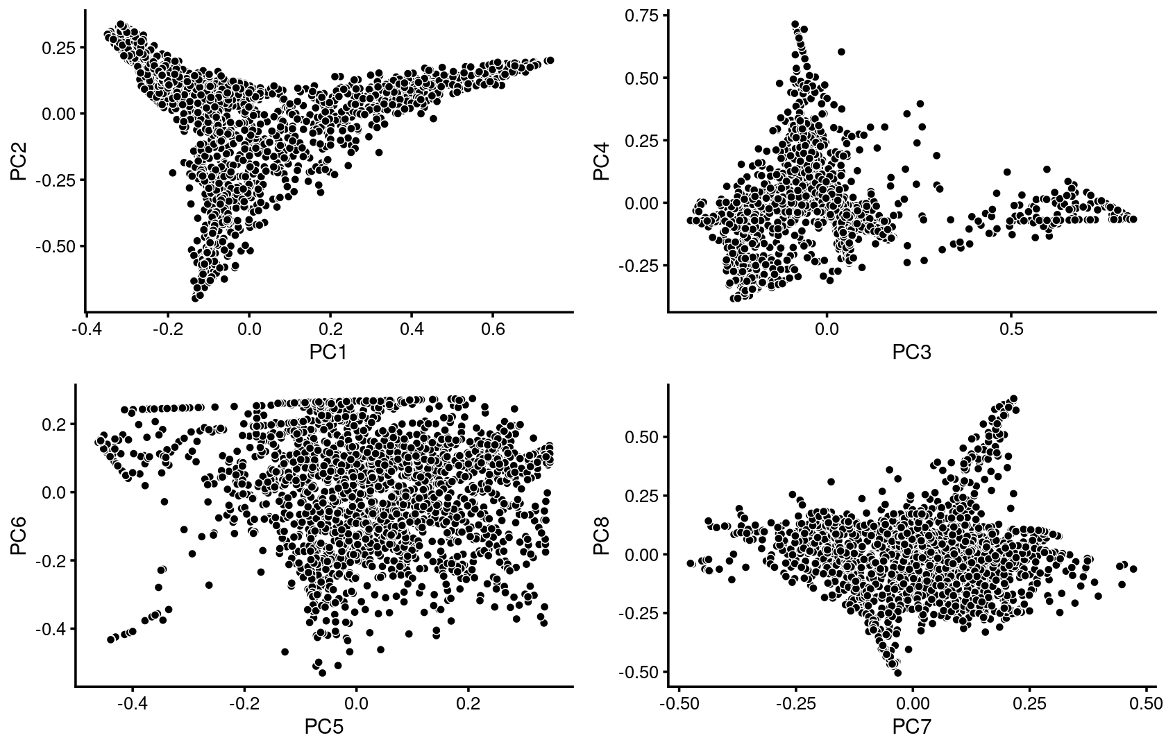
| Version | Author | Date |
|---|---|---|
| fb6a121 | kevinlkx | 2020-11-06 |
Some of the structure is more evident from “hexbin” plots showing the density of the points.
breaks <- c(0,1,5,10,100,Inf)
p.pca2.1 <- pca_hexbin_plot(poisson2multinom(fit), pcs = 1:2, breaks = breaks) + guides(fill = "none")
p.pca2.2 <- pca_hexbin_plot(poisson2multinom(fit), pcs = 3:4, breaks = breaks) + guides(fill = "none")
p.pca2.3 <- pca_hexbin_plot(poisson2multinom(fit), pcs = 5:6, breaks = breaks) + guides(fill = "none")
p.pca2.4 <- pca_hexbin_plot(poisson2multinom(fit), pcs = 7:8, breaks = breaks) + guides(fill = "none")

plot_grid(p.pca2.1,p.pca2.2,p.pca2.3,p.pca2.4)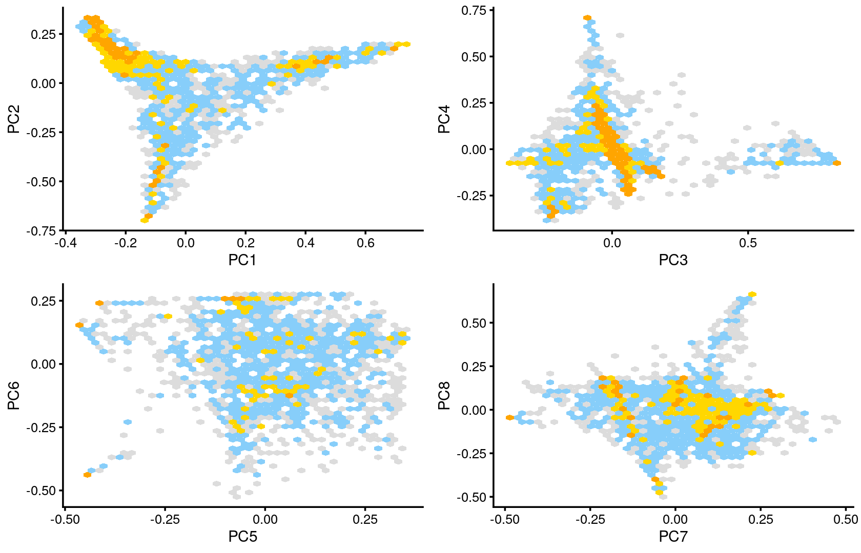
| Version | Author | Date |
|---|---|---|
| fb6a121 | kevinlkx | 2020-11-06 |
Next, we layer the cell labels onto the PC plots.
p.pca3.1 <- labeled_pca_plot(fit,1:2,samples$label,font_size = 7,
                       legend_label = "Cell labels")
p.pca3.2 <- labeled_pca_plot(fit,3:4,samples$label,font_size = 7,
                       legend_label = "Cell labels")
p.pca3.3 <- labeled_pca_plot(fit,5:6,samples$label,font_size = 7,
                       legend_label = "Cell labels")
p.pca3.4 <- labeled_pca_plot(fit,7:8,samples$label,font_size = 7,
                       legend_label = "Cell labels")

plot_grid(p.pca3.1,p.pca3.2,p.pca3.3,p.pca3.4)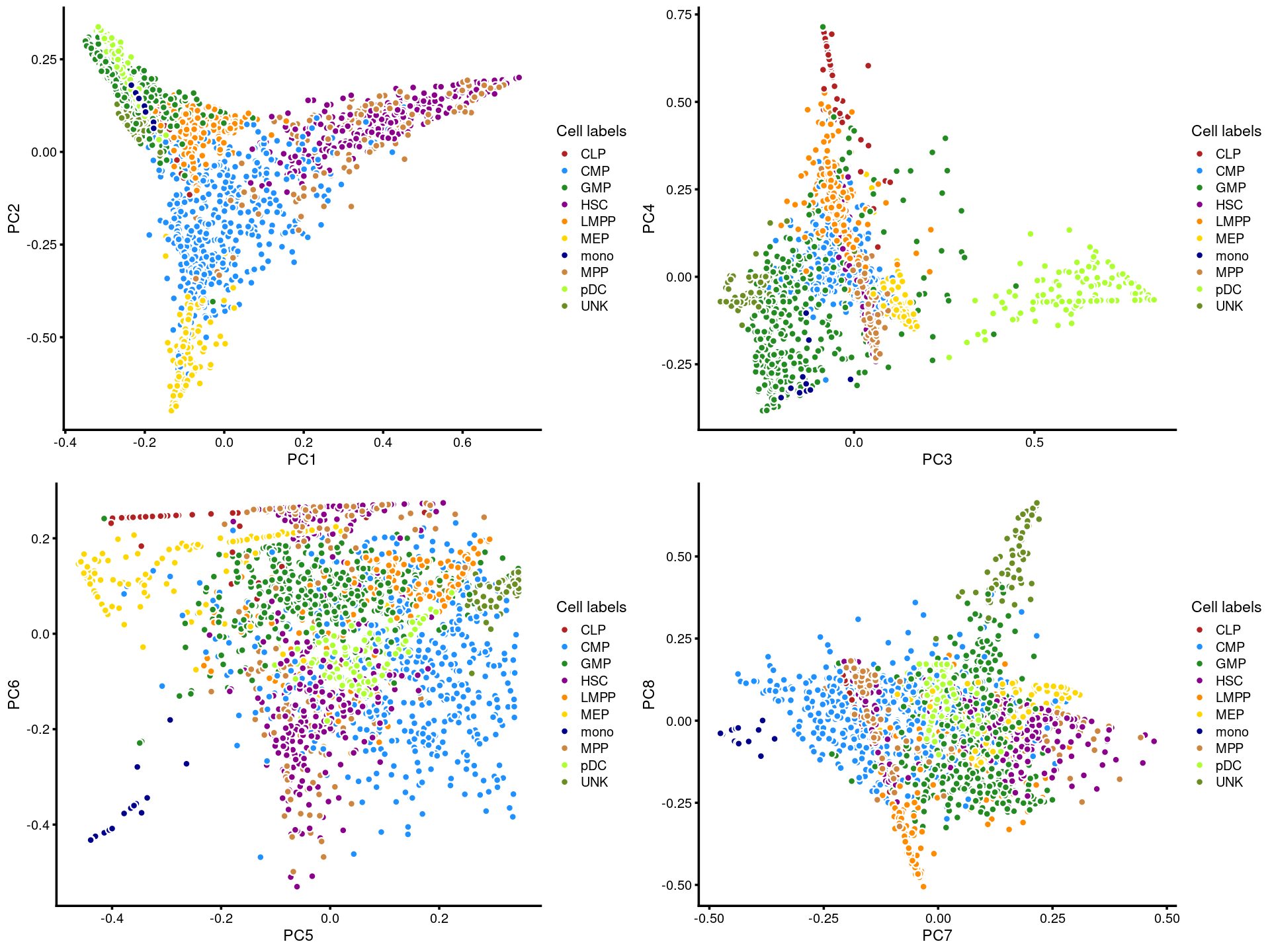
| Version | Author | Date |
|---|---|---|
| fb6a121 | kevinlkx | 2020-11-06 |
k = 12
Load the \(k = 12\) Poisson NMF fit.
out.dir <- "/project2/mstephens/kevinluo/scATACseq-topics/output/Buenrostro_2018/unbinarized/"
fit <- readRDS(file.path(out.dir, "/fit-Buenrostro2018-scd-ex-k=12.rds"))$fit
Plot PCs of the topic proportions.
p.pca1.1 <- pca_plot(poisson2multinom(fit),pcs = 1:2,fill = "none")
p.pca1.2 <- pca_plot(poisson2multinom(fit),pcs = 3:4,fill = "none")
p.pca1.3 <- pca_plot(poisson2multinom(fit),pcs = 5:6,fill = "none")
p.pca1.4 <- pca_plot(poisson2multinom(fit),pcs = 7:8,fill = "none")

plot_grid(p.pca1.1,p.pca1.2,p.pca1.3,p.pca1.4)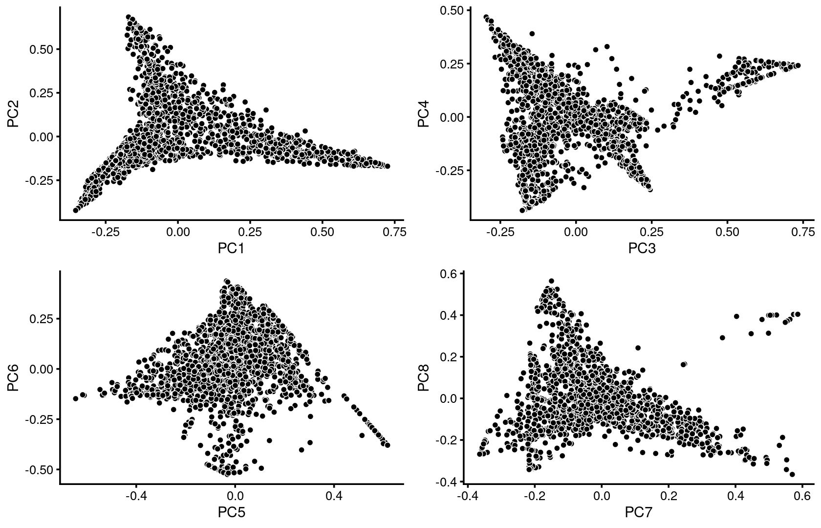
| Version | Author | Date |
|---|---|---|
| fb6a121 | kevinlkx | 2020-11-06 |
Some of the structure is more evident from “hexbin” plots showing the density of the points.
breaks <- c(0,1,5,10,100,Inf)
p.pca2.1 <- pca_hexbin_plot(poisson2multinom(fit), pcs = 1:2, breaks = breaks) + guides(fill = "none")
p.pca2.2 <- pca_hexbin_plot(poisson2multinom(fit), pcs = 3:4, breaks = breaks) + guides(fill = "none")
p.pca2.3 <- pca_hexbin_plot(poisson2multinom(fit), pcs = 5:6, breaks = breaks) + guides(fill = "none")
p.pca2.4 <- pca_hexbin_plot(poisson2multinom(fit), pcs = 7:8, breaks = breaks) + guides(fill = "none")

plot_grid(p.pca2.1,p.pca2.2,p.pca2.3,p.pca2.4)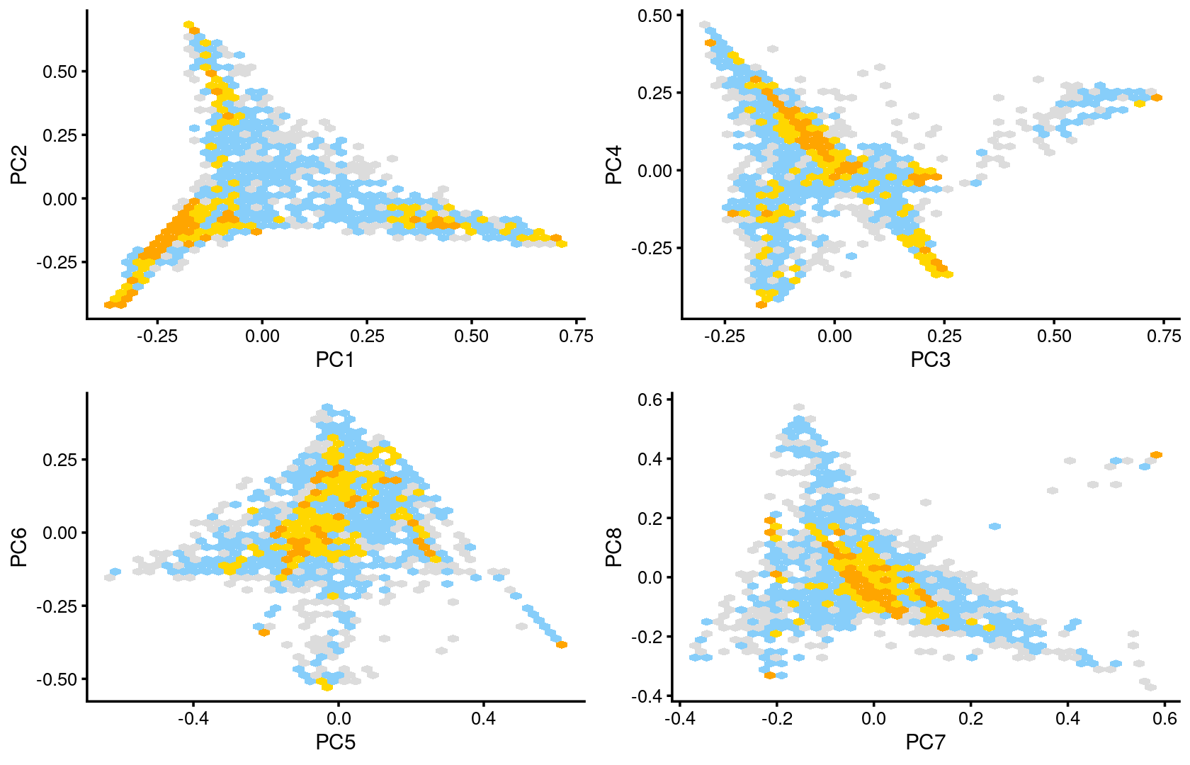
| Version | Author | Date |
|---|---|---|
| fb6a121 | kevinlkx | 2020-11-06 |
Next, we layer the cell labels onto the PC plots.
p.pca3.1 <- labeled_pca_plot(fit,1:2,samples$label,font_size = 7,
                       legend_label = "Cell labels")
p.pca3.2 <- labeled_pca_plot(fit,3:4,samples$label,font_size = 7,
                       legend_label = "Cell labels")
p.pca3.3 <- labeled_pca_plot(fit,5:6,samples$label,font_size = 7,
                       legend_label = "Cell labels")
p.pca3.4 <- labeled_pca_plot(fit,7:8,samples$label,font_size = 7,
                       legend_label = "Cell labels")

plot_grid(p.pca3.1,p.pca3.2,p.pca3.3,p.pca3.4)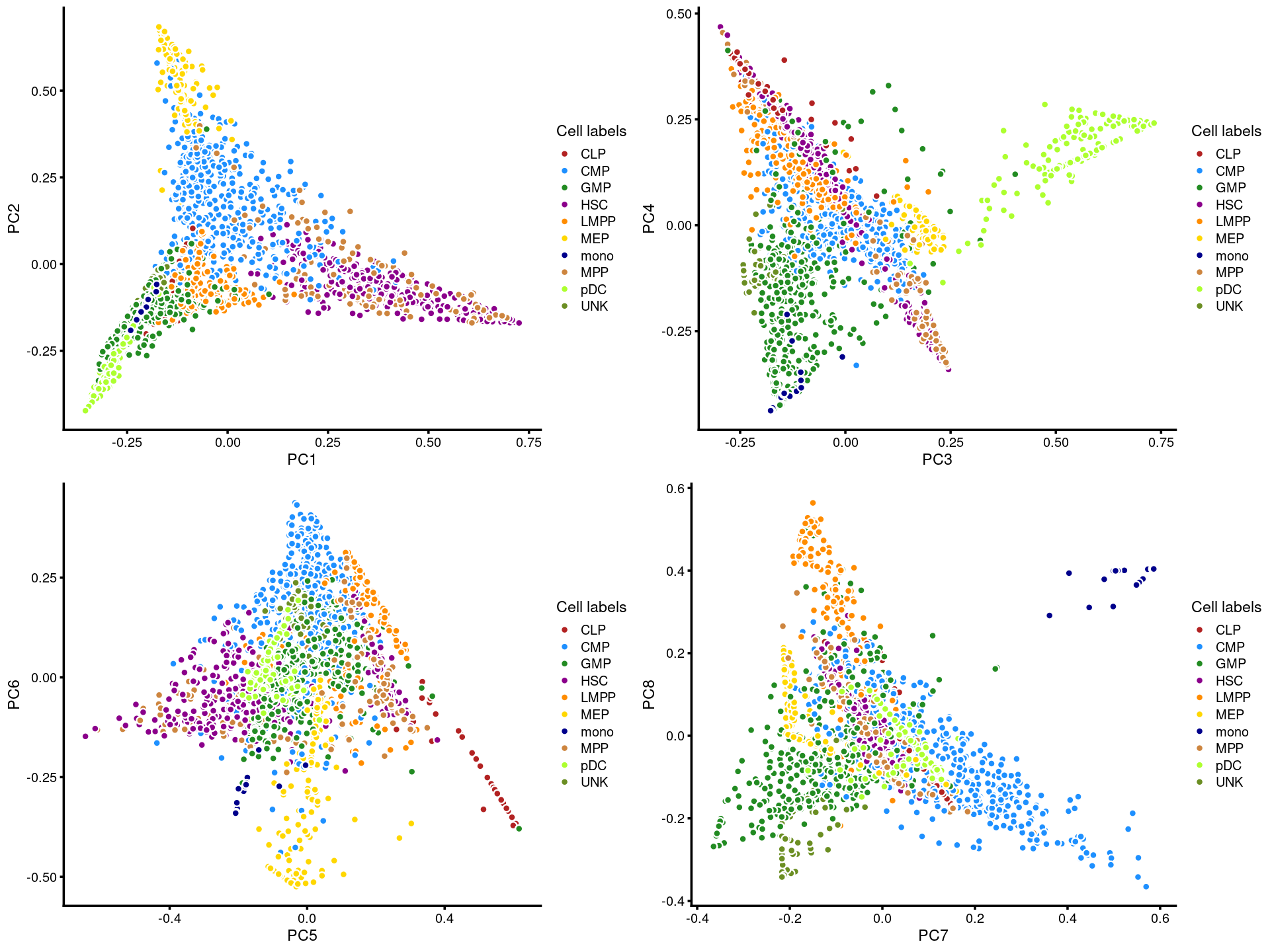
| Version | Author | Date |
|---|---|---|
| fb6a121 | kevinlkx | 2020-11-06 |
k = 13
Load the \(k = 13\) Poisson NMF fit.
out.dir <- "/project2/mstephens/kevinluo/scATACseq-topics/output/Buenrostro_2018/unbinarized/"
fit <- readRDS(file.path(out.dir, "/fit-Buenrostro2018-scd-ex-k=13.rds"))$fit
Plot PCs of the topic proportions.
p.pca1.1 <- pca_plot(poisson2multinom(fit),pcs = 1:2,fill = "none")
p.pca1.2 <- pca_plot(poisson2multinom(fit),pcs = 3:4,fill = "none")
p.pca1.3 <- pca_plot(poisson2multinom(fit),pcs = 5:6,fill = "none")
p.pca1.4 <- pca_plot(poisson2multinom(fit),pcs = 7:8,fill = "none")

plot_grid(p.pca1.1,p.pca1.2,p.pca1.3,p.pca1.4)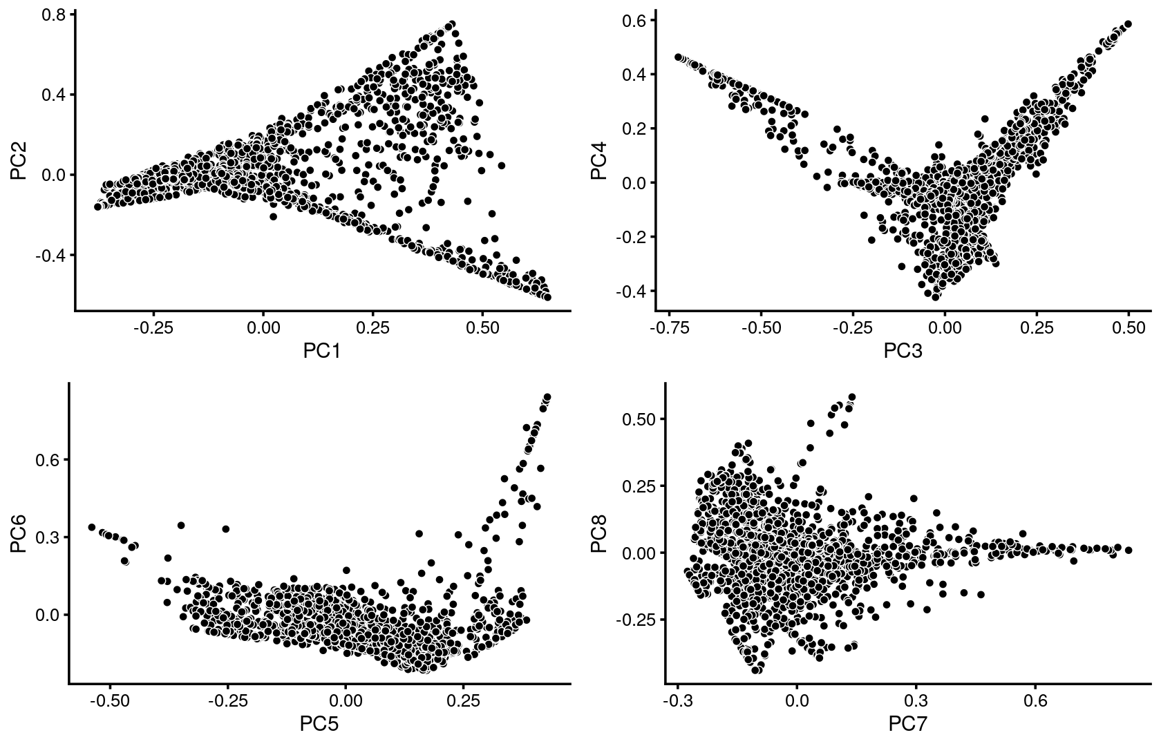
| Version | Author | Date |
|---|---|---|
| fb6a121 | kevinlkx | 2020-11-06 |
Some of the structure is more evident from “hexbin” plots showing the density of the points.
breaks <- c(0,1,5,10,100,Inf)
p.pca2.1 <- pca_hexbin_plot(poisson2multinom(fit), pcs = 1:2, breaks = breaks) + guides(fill = "none")
p.pca2.2 <- pca_hexbin_plot(poisson2multinom(fit), pcs = 3:4, breaks = breaks) + guides(fill = "none")
p.pca2.3 <- pca_hexbin_plot(poisson2multinom(fit), pcs = 5:6, breaks = breaks) + guides(fill = "none")
p.pca2.4 <- pca_hexbin_plot(poisson2multinom(fit), pcs = 7:8, breaks = breaks) + guides(fill = "none")

plot_grid(p.pca2.1,p.pca2.2,p.pca2.3,p.pca2.4)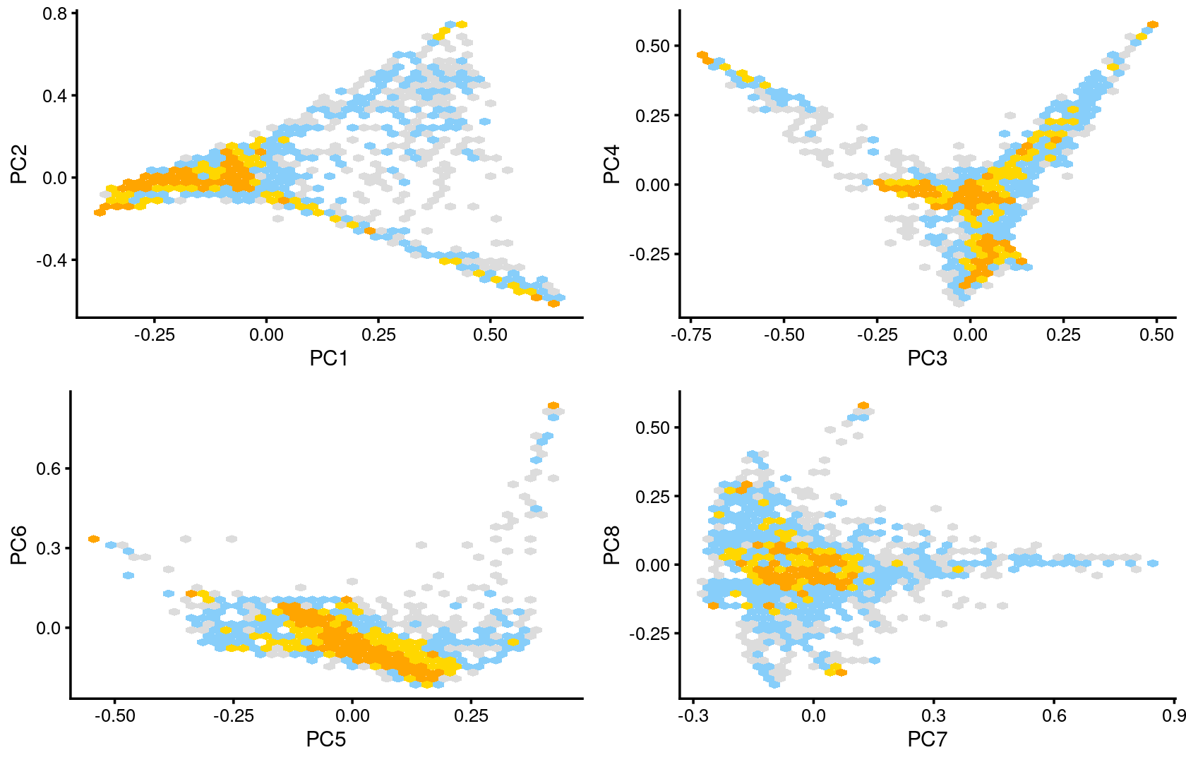
| Version | Author | Date |
|---|---|---|
| fb6a121 | kevinlkx | 2020-11-06 |
Next, we layer the cell labels onto the PC plots.
p.pca3.1 <- labeled_pca_plot(fit,1:2,samples$label,font_size = 7,
                       legend_label = "Cell labels")
p.pca3.2 <- labeled_pca_plot(fit,3:4,samples$label,font_size = 7,
                       legend_label = "Cell labels")
p.pca3.3 <- labeled_pca_plot(fit,5:6,samples$label,font_size = 7,
                       legend_label = "Cell labels")
p.pca3.4 <- labeled_pca_plot(fit,7:8,samples$label,font_size = 7,
                       legend_label = "Cell labels")

plot_grid(p.pca3.1,p.pca3.2,p.pca3.3,p.pca3.4)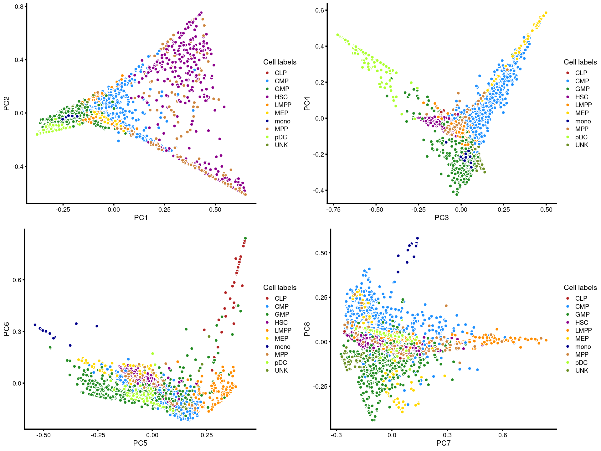
| Version | Author | Date |
|---|---|---|
| fb6a121 | kevinlkx | 2020-11-06 |
k = 14
Load the \(k = 14\) Poisson NMF fit.
out.dir <- "/project2/mstephens/kevinluo/scATACseq-topics/output/Buenrostro_2018/unbinarized/"
fit <- readRDS(file.path(out.dir, "/fit-Buenrostro2018-scd-ex-k=14.rds"))$fit
Plot PCs of the topic proportions.
p.pca1.1 <- pca_plot(poisson2multinom(fit),pcs = 1:2,fill = "none")
p.pca1.2 <- pca_plot(poisson2multinom(fit),pcs = 3:4,fill = "none")
p.pca1.3 <- pca_plot(poisson2multinom(fit),pcs = 5:6,fill = "none")
p.pca1.4 <- pca_plot(poisson2multinom(fit),pcs = 7:8,fill = "none")

plot_grid(p.pca1.1,p.pca1.2,p.pca1.3,p.pca1.4)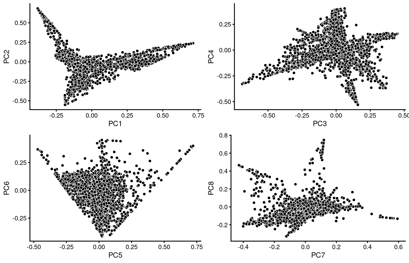
| Version | Author | Date |
|---|---|---|
| fb6a121 | kevinlkx | 2020-11-06 |
Some of the structure is more evident from “hexbin” plots showing the density of the points.
breaks <- c(0,1,5,10,100,Inf)
p.pca2.1 <- pca_hexbin_plot(poisson2multinom(fit), pcs = 1:2, breaks = breaks) + guides(fill = "none")
p.pca2.2 <- pca_hexbin_plot(poisson2multinom(fit), pcs = 3:4, breaks = breaks) + guides(fill = "none")
p.pca2.3 <- pca_hexbin_plot(poisson2multinom(fit), pcs = 5:6, breaks = breaks) + guides(fill = "none")
p.pca2.4 <- pca_hexbin_plot(poisson2multinom(fit), pcs = 7:8, breaks = breaks) + guides(fill = "none")

plot_grid(p.pca2.1,p.pca2.2,p.pca2.3,p.pca2.4)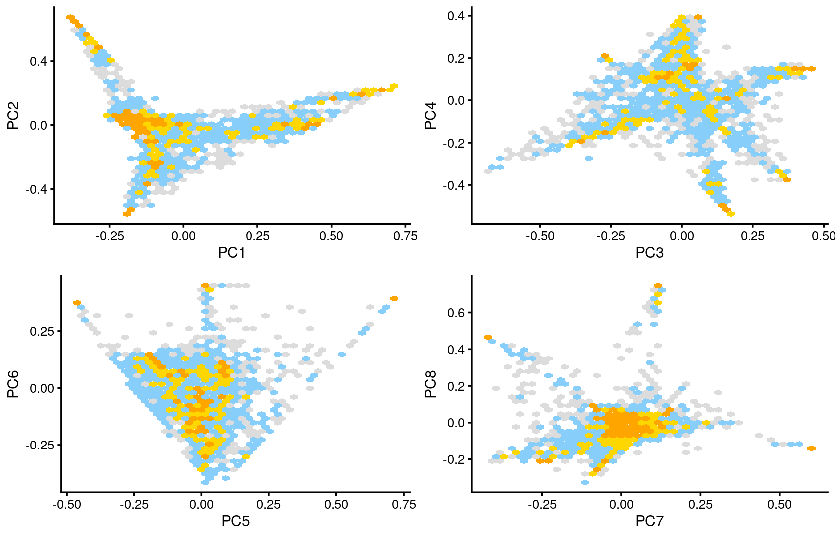
| Version | Author | Date |
|---|---|---|
| fb6a121 | kevinlkx | 2020-11-06 |
Next, we layer the cell labels onto the PC plots.
p.pca3.1 <- labeled_pca_plot(fit,1:2,samples$label,font_size = 7,
                       legend_label = "Cell labels")
p.pca3.2 <- labeled_pca_plot(fit,3:4,samples$label,font_size = 7,
                       legend_label = "Cell labels")
p.pca3.3 <- labeled_pca_plot(fit,5:6,samples$label,font_size = 7,
                       legend_label = "Cell labels")
p.pca3.4 <- labeled_pca_plot(fit,7:8,samples$label,font_size = 7,
                       legend_label = "Cell labels")

plot_grid(p.pca3.1,p.pca3.2,p.pca3.3,p.pca3.4)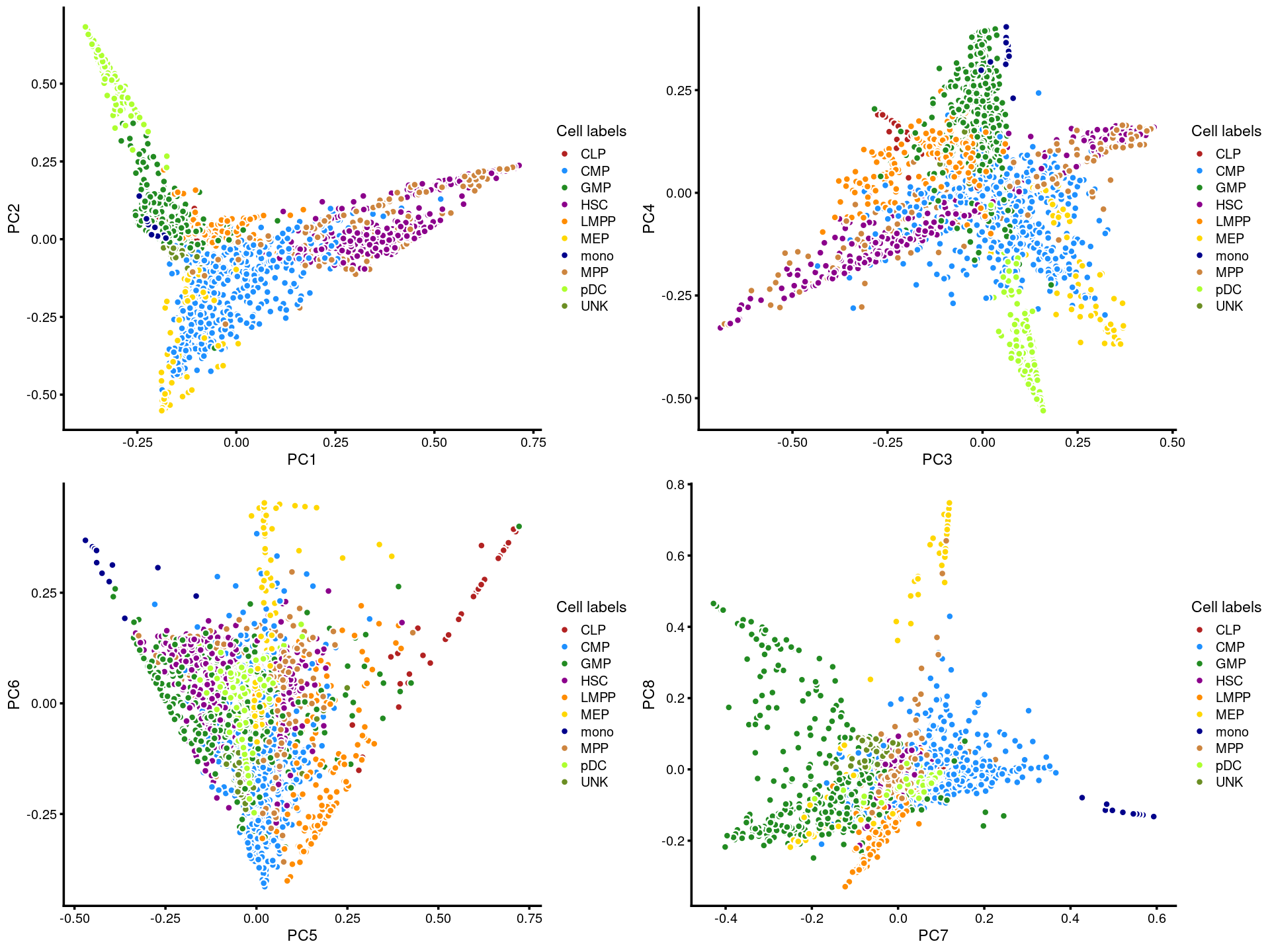
| Version | Author | Date |
|---|---|---|
| fb6a121 | kevinlkx | 2020-11-06 |
k = 15
Load the \(k = 15\) Poisson NMF fit.
out.dir <- "/project2/mstephens/kevinluo/scATACseq-topics/output/Buenrostro_2018/unbinarized/"
fit <- readRDS(file.path(out.dir, "/fit-Buenrostro2018-scd-ex-k=15.rds"))$fit
Plot PCs of the topic proportions.
p.pca1.1 <- pca_plot(poisson2multinom(fit),pcs = 1:2,fill = "none")
p.pca1.2 <- pca_plot(poisson2multinom(fit),pcs = 3:4,fill = "none")
p.pca1.3 <- pca_plot(poisson2multinom(fit),pcs = 5:6,fill = "none")
p.pca1.4 <- pca_plot(poisson2multinom(fit),pcs = 7:8,fill = "none")

plot_grid(p.pca1.1,p.pca1.2,p.pca1.3,p.pca1.4)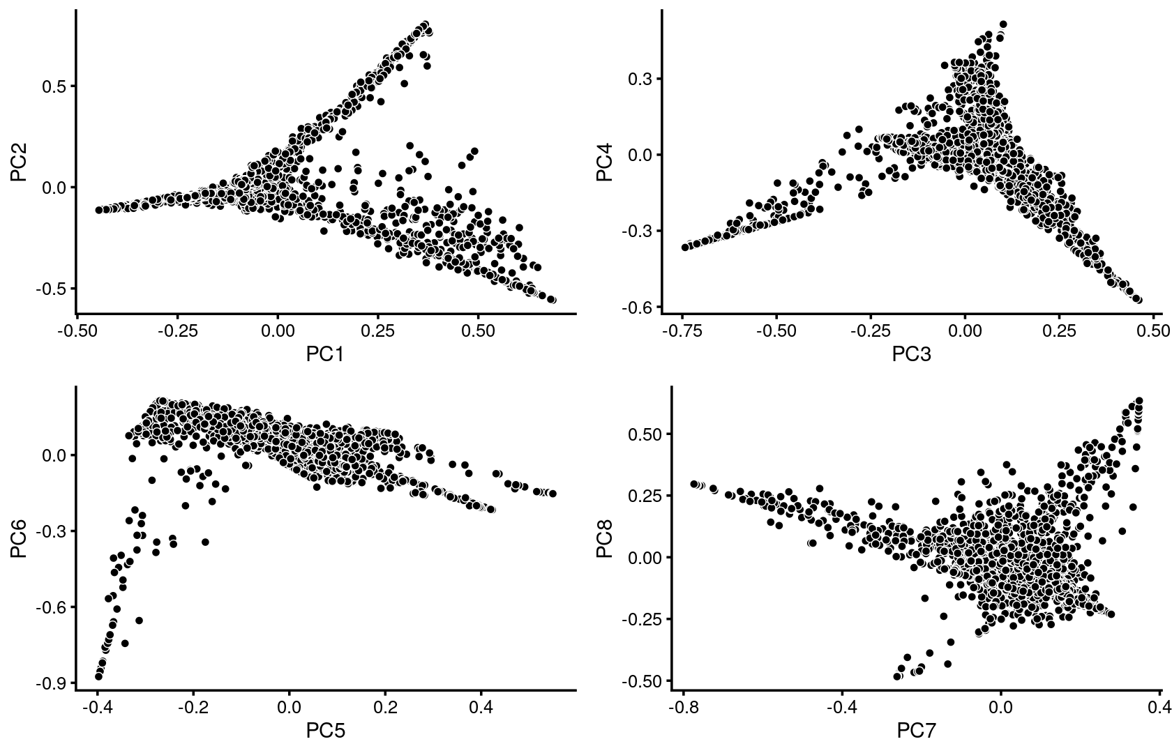
| Version | Author | Date |
|---|---|---|
| fb6a121 | kevinlkx | 2020-11-06 |
Some of the structure is more evident from “hexbin” plots showing the density of the points.
breaks <- c(0,1,5,10,100,Inf)
p.pca2.1 <- pca_hexbin_plot(poisson2multinom(fit), pcs = 1:2, breaks = breaks) + guides(fill = "none")
p.pca2.2 <- pca_hexbin_plot(poisson2multinom(fit), pcs = 3:4, breaks = breaks) + guides(fill = "none")
p.pca2.3 <- pca_hexbin_plot(poisson2multinom(fit), pcs = 5:6, breaks = breaks) + guides(fill = "none")
p.pca2.4 <- pca_hexbin_plot(poisson2multinom(fit), pcs = 7:8, breaks = breaks) + guides(fill = "none")

plot_grid(p.pca2.1,p.pca2.2,p.pca2.3,p.pca2.4)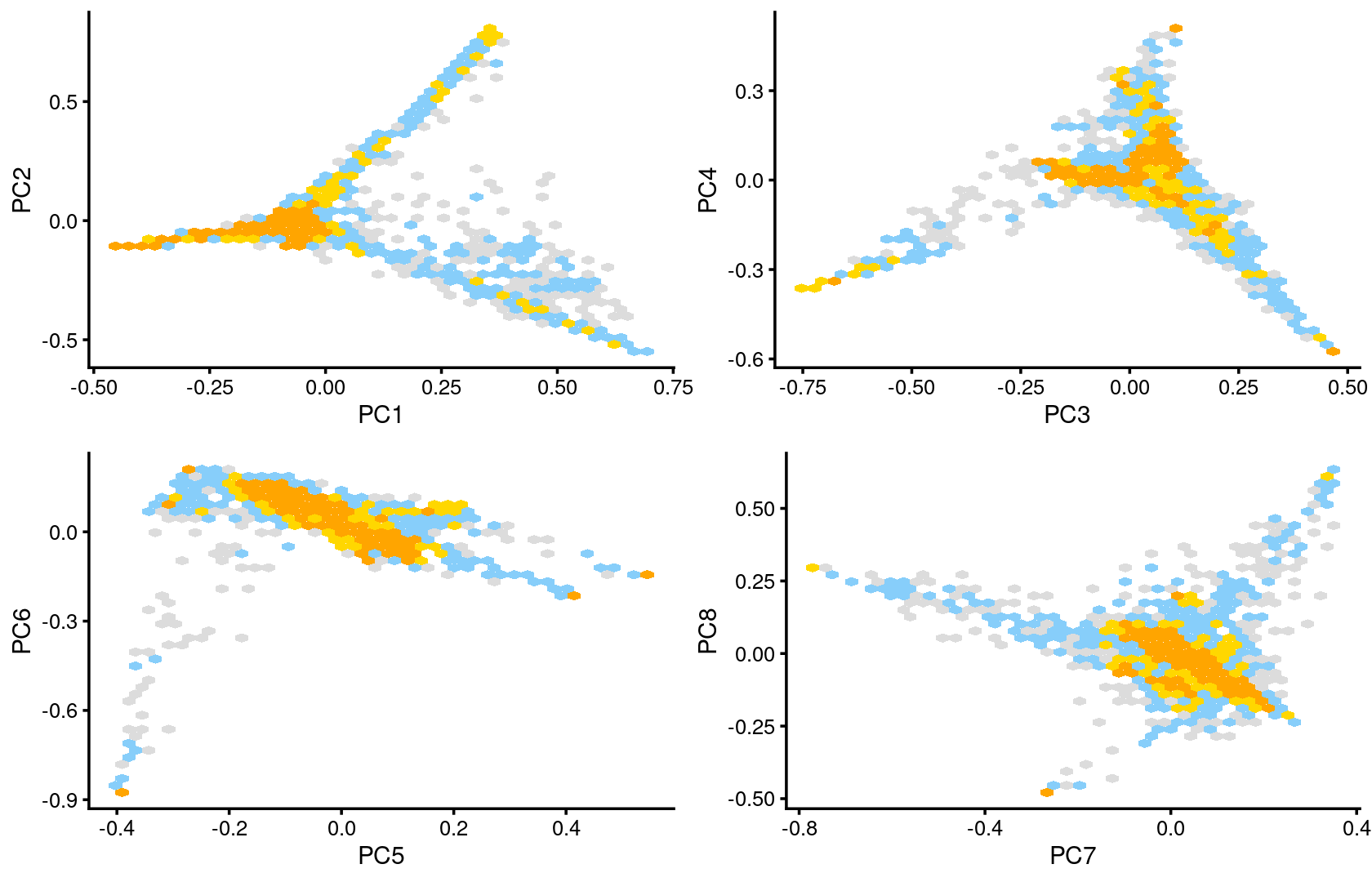
| Version | Author | Date |
|---|---|---|
| fb6a121 | kevinlkx | 2020-11-06 |
Next, we layer the cell labels onto the PC plots.
p.pca3.1 <- labeled_pca_plot(fit,1:2,samples$label,font_size = 7,
                       legend_label = "Cell labels")
p.pca3.2 <- labeled_pca_plot(fit,3:4,samples$label,font_size = 7,
                       legend_label = "Cell labels")
p.pca3.3 <- labeled_pca_plot(fit,5:6,samples$label,font_size = 7,
                       legend_label = "Cell labels")
p.pca3.4 <- labeled_pca_plot(fit,7:8,samples$label,font_size = 7,
                       legend_label = "Cell labels")

plot_grid(p.pca3.1,p.pca3.2,p.pca3.3,p.pca3.4)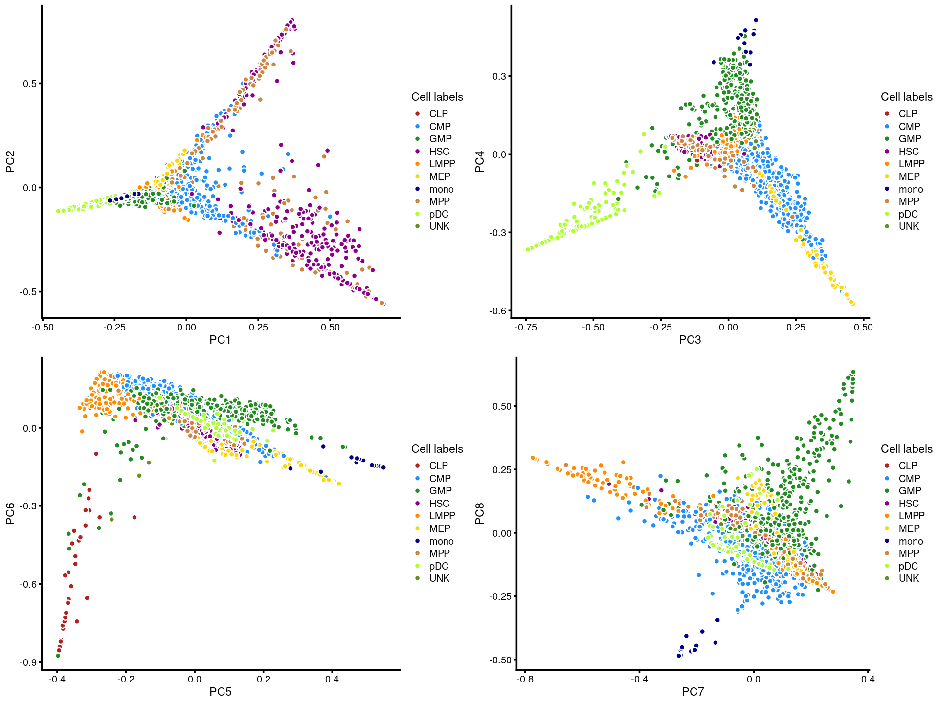
| Version | Author | Date |
|---|---|---|
| fb6a121 | kevinlkx | 2020-11-06 |
Binarized counts
Load the data
data.dir <- "/project2/mstephens/kevinluo/scATACseq-topics/data/Buenrostro_2018/processed_data/"
load(file.path(data.dir, "Buenrostro_2018_counts.RData"))
cat(sprintf("%d x %d counts matrix.\n",nrow(counts),ncol(counts)))
rm(counts)
samples$label <- as.factor(samples$label)
# 2034 x 101172 counts matrix.
Plot PCs of the topic proportions
We first use PCA to explore the structure inferred from the multinomial topic model with different numbers of \(k\):
k = 10
Load the \(k = 10\) Poisson NMF fit.
out.dir <- "/project2/mstephens/kevinluo/scATACseq-topics/output/Buenrostro_2018/binarized/"
fit <- readRDS(file.path(out.dir, "/fit-Buenrostro2018-binarized-scd-ex-k=10.rds"))$fit
Plot PCs of the topic proportions.
p.pca1.1 <- pca_plot(poisson2multinom(fit),pcs = 1:2,fill = "none")
p.pca1.2 <- pca_plot(poisson2multinom(fit),pcs = 3:4,fill = "none")
p.pca1.3 <- pca_plot(poisson2multinom(fit),pcs = 5:6,fill = "none")
p.pca1.4 <- pca_plot(poisson2multinom(fit),pcs = 7:8,fill = "none")

plot_grid(p.pca1.1,p.pca1.2,p.pca1.3,p.pca1.4)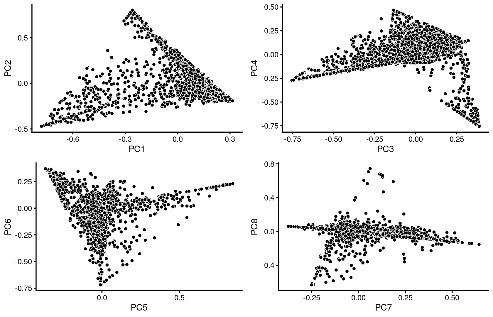
| Version | Author | Date |
|---|---|---|
| fb6a121 | kevinlkx | 2020-11-06 |
Some of the structure is more evident from “hexbin” plots showing the density of the points.
breaks <- c(0,1,5,10,100,Inf)
p.pca2.1 <- pca_hexbin_plot(poisson2multinom(fit), pcs = 1:2, breaks = breaks) + guides(fill = "none")
p.pca2.2 <- pca_hexbin_plot(poisson2multinom(fit), pcs = 3:4, breaks = breaks) + guides(fill = "none")
p.pca2.3 <- pca_hexbin_plot(poisson2multinom(fit), pcs = 5:6, breaks = breaks) + guides(fill = "none")
p.pca2.4 <- pca_hexbin_plot(poisson2multinom(fit), pcs = 7:8, breaks = breaks) + guides(fill = "none")

plot_grid(p.pca2.1,p.pca2.2,p.pca2.3,p.pca2.4)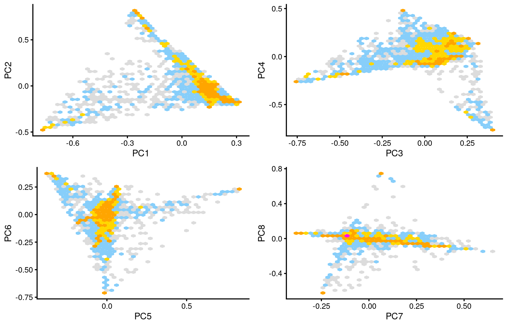
| Version | Author | Date |
|---|---|---|
| fb6a121 | kevinlkx | 2020-11-06 |
Next, we layer the cell labels onto the PC plots.
p.pca3.1 <- labeled_pca_plot(fit,1:2,samples$label,font_size = 7,
                       legend_label = "Cell labels")
p.pca3.2 <- labeled_pca_plot(fit,3:4,samples$label,font_size = 7,
                       legend_label = "Cell labels")
p.pca3.3 <- labeled_pca_plot(fit,5:6,samples$label,font_size = 7,
                       legend_label = "Cell labels")
p.pca3.4 <- labeled_pca_plot(fit,7:8,samples$label,font_size = 7,
                       legend_label = "Cell labels")

plot_grid(p.pca3.1,p.pca3.2,p.pca3.3,p.pca3.4)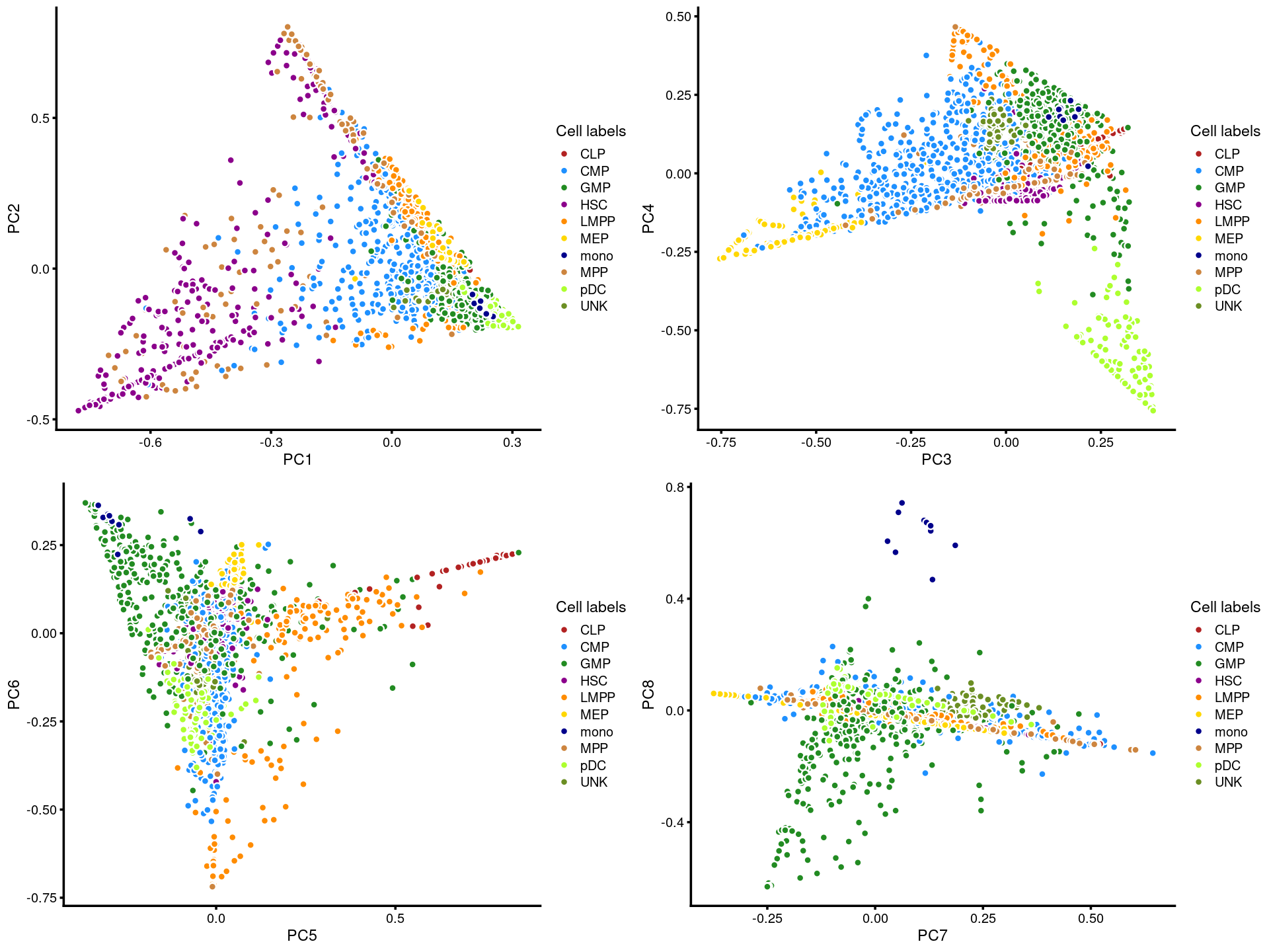
| Version | Author | Date |
|---|---|---|
| fb6a121 | kevinlkx | 2020-11-06 |
k = 11
Load the \(k = 11\) Poisson NMF fit.
out.dir <- "/project2/mstephens/kevinluo/scATACseq-topics/output/Buenrostro_2018/binarized/"
fit <- readRDS(file.path(out.dir, "/fit-Buenrostro2018-binarized-scd-ex-k=11.rds"))$fit
Plot PCs of the topic proportions.
p.pca1.1 <- pca_plot(poisson2multinom(fit),pcs = 1:2,fill = "none")
p.pca1.2 <- pca_plot(poisson2multinom(fit),pcs = 3:4,fill = "none")
p.pca1.3 <- pca_plot(poisson2multinom(fit),pcs = 5:6,fill = "none")
p.pca1.4 <- pca_plot(poisson2multinom(fit),pcs = 7:8,fill = "none")

plot_grid(p.pca1.1,p.pca1.2,p.pca1.3,p.pca1.4)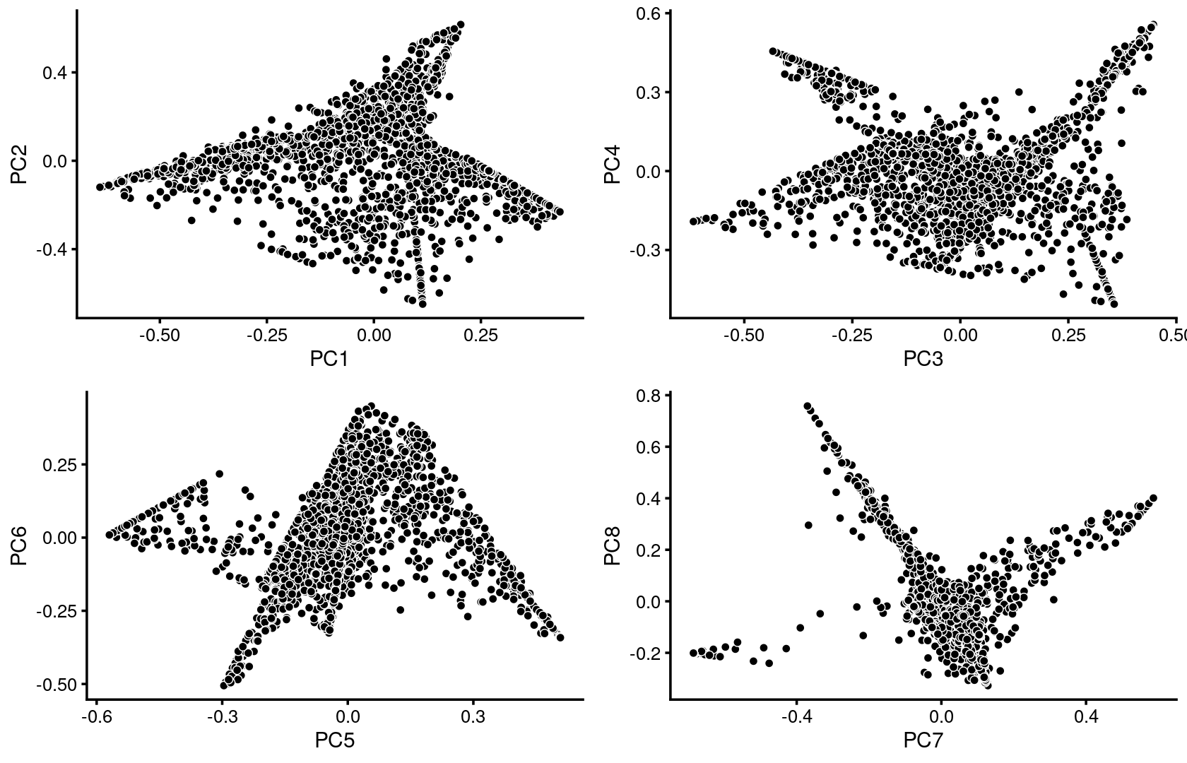
| Version | Author | Date |
|---|---|---|
| fb6a121 | kevinlkx | 2020-11-06 |
Some of the structure is more evident from “hexbin” plots showing the density of the points.
breaks <- c(0,1,5,10,100,Inf)
p.pca2.1 <- pca_hexbin_plot(poisson2multinom(fit), pcs = 1:2, breaks = breaks) + guides(fill = "none")
p.pca2.2 <- pca_hexbin_plot(poisson2multinom(fit), pcs = 3:4, breaks = breaks) + guides(fill = "none")
p.pca2.3 <- pca_hexbin_plot(poisson2multinom(fit), pcs = 5:6, breaks = breaks) + guides(fill = "none")
p.pca2.4 <- pca_hexbin_plot(poisson2multinom(fit), pcs = 7:8, breaks = breaks) + guides(fill = "none")

plot_grid(p.pca2.1,p.pca2.2,p.pca2.3,p.pca2.4)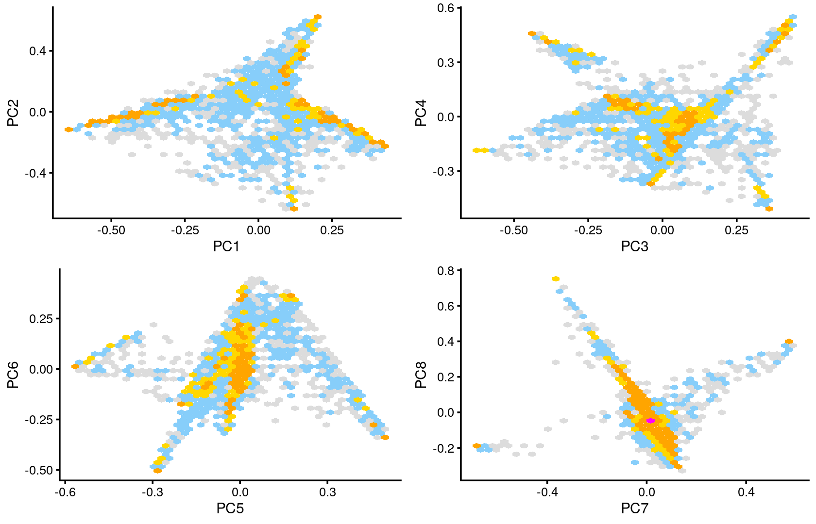
| Version | Author | Date |
|---|---|---|
| fb6a121 | kevinlkx | 2020-11-06 |
Next, we layer the cell labels onto the PC plots.
p.pca3.1 <- labeled_pca_plot(fit,1:2,samples$label,font_size = 7,
                       legend_label = "Cell labels")
p.pca3.2 <- labeled_pca_plot(fit,3:4,samples$label,font_size = 7,
                       legend_label = "Cell labels")
p.pca3.3 <- labeled_pca_plot(fit,5:6,samples$label,font_size = 7,
                       legend_label = "Cell labels")
p.pca3.4 <- labeled_pca_plot(fit,7:8,samples$label,font_size = 7,
                       legend_label = "Cell labels")

plot_grid(p.pca3.1,p.pca3.2,p.pca3.3,p.pca3.4)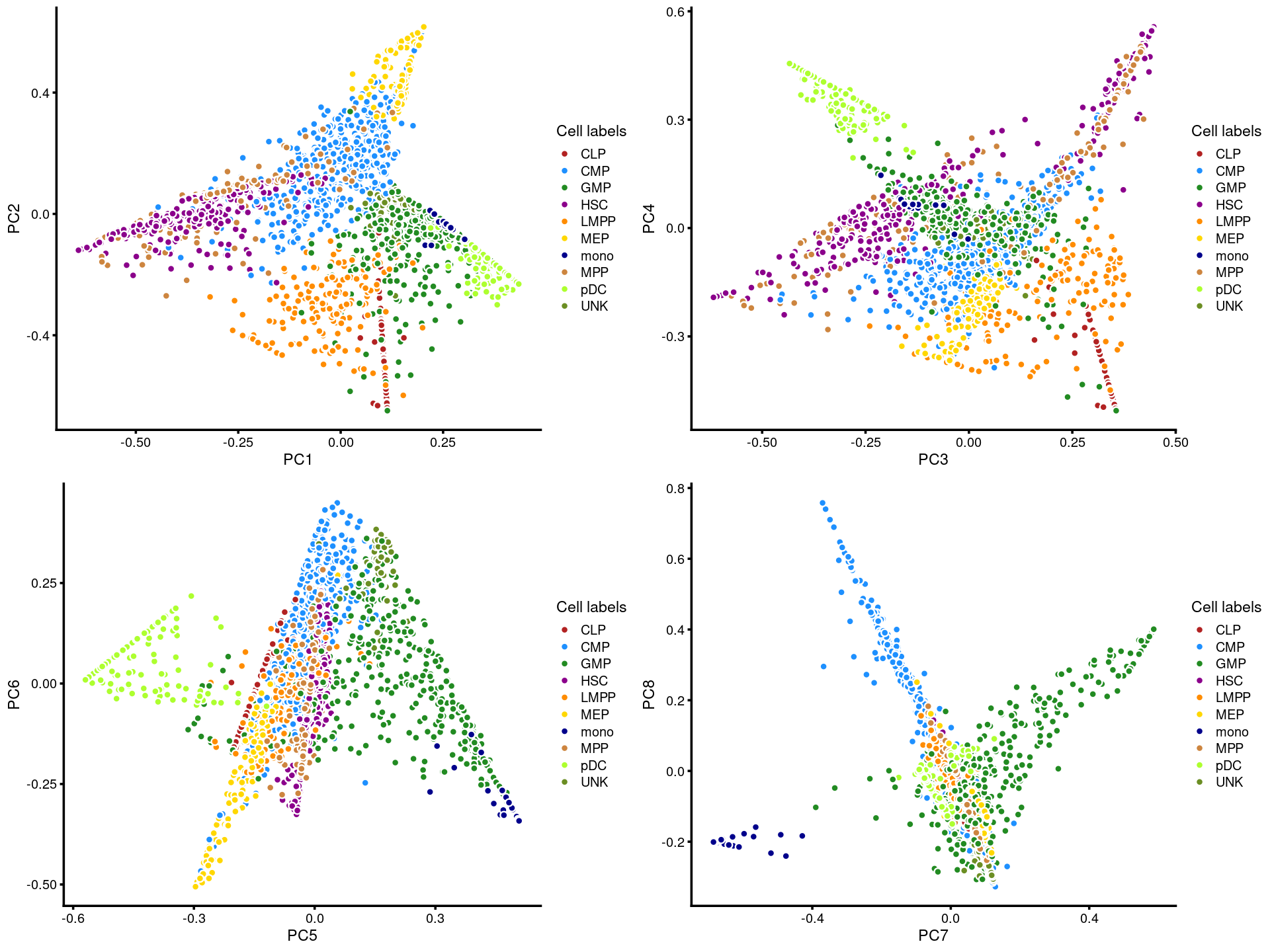
| Version | Author | Date |
|---|---|---|
| fb6a121 | kevinlkx | 2020-11-06 |
k = 12
Load the \(k = 12\) Poisson NMF fit.
out.dir <- "/project2/mstephens/kevinluo/scATACseq-topics/output/Buenrostro_2018/binarized/"
fit <- readRDS(file.path(out.dir, "/fit-Buenrostro2018-binarized-scd-ex-k=12.rds"))$fit
Plot PCs of the topic proportions.
p.pca1.1 <- pca_plot(poisson2multinom(fit),pcs = 1:2,fill = "none")
p.pca1.2 <- pca_plot(poisson2multinom(fit),pcs = 3:4,fill = "none")
p.pca1.3 <- pca_plot(poisson2multinom(fit),pcs = 5:6,fill = "none")
p.pca1.4 <- pca_plot(poisson2multinom(fit),pcs = 7:8,fill = "none")

plot_grid(p.pca1.1,p.pca1.2,p.pca1.3,p.pca1.4)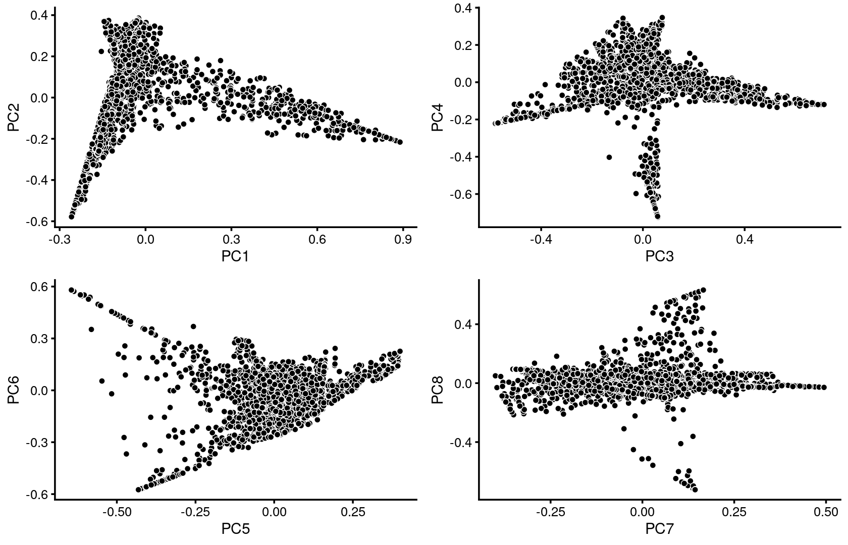
| Version | Author | Date |
|---|---|---|
| fb6a121 | kevinlkx | 2020-11-06 |
Some of the structure is more evident from “hexbin” plots showing the density of the points.
breaks <- c(0,1,5,10,100,Inf)
p.pca2.1 <- pca_hexbin_plot(poisson2multinom(fit), pcs = 1:2, breaks = breaks) + guides(fill = "none")
p.pca2.2 <- pca_hexbin_plot(poisson2multinom(fit), pcs = 3:4, breaks = breaks) + guides(fill = "none")
p.pca2.3 <- pca_hexbin_plot(poisson2multinom(fit), pcs = 5:6, breaks = breaks) + guides(fill = "none")
p.pca2.4 <- pca_hexbin_plot(poisson2multinom(fit), pcs = 7:8, breaks = breaks) + guides(fill = "none")

plot_grid(p.pca2.1,p.pca2.2,p.pca2.3,p.pca2.4)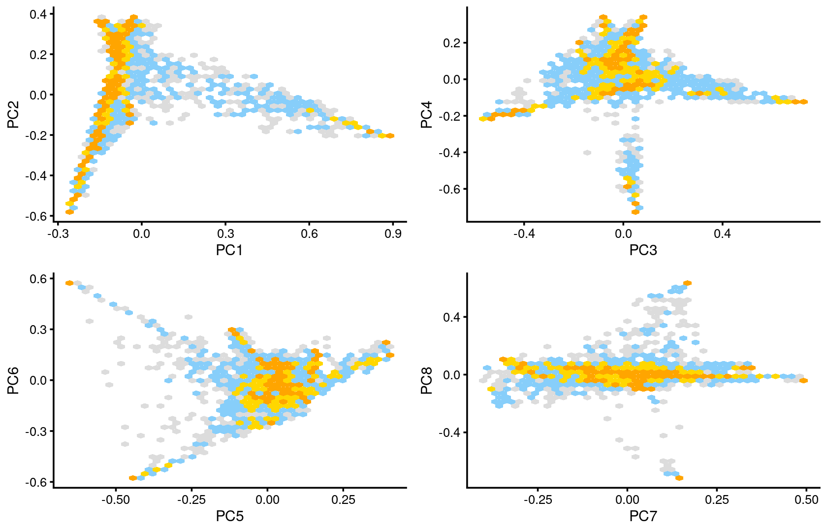
| Version | Author | Date |
|---|---|---|
| fb6a121 | kevinlkx | 2020-11-06 |
Next, we layer the cell labels onto the PC plots.
p.pca3.1 <- labeled_pca_plot(fit,1:2,samples$label,font_size = 7,
                       legend_label = "Cell labels")
p.pca3.2 <- labeled_pca_plot(fit,3:4,samples$label,font_size = 7,
                       legend_label = "Cell labels")
p.pca3.3 <- labeled_pca_plot(fit,5:6,samples$label,font_size = 7,
                       legend_label = "Cell labels")
p.pca3.4 <- labeled_pca_plot(fit,7:8,samples$label,font_size = 7,
                       legend_label = "Cell labels")

plot_grid(p.pca3.1,p.pca3.2,p.pca3.3,p.pca3.4)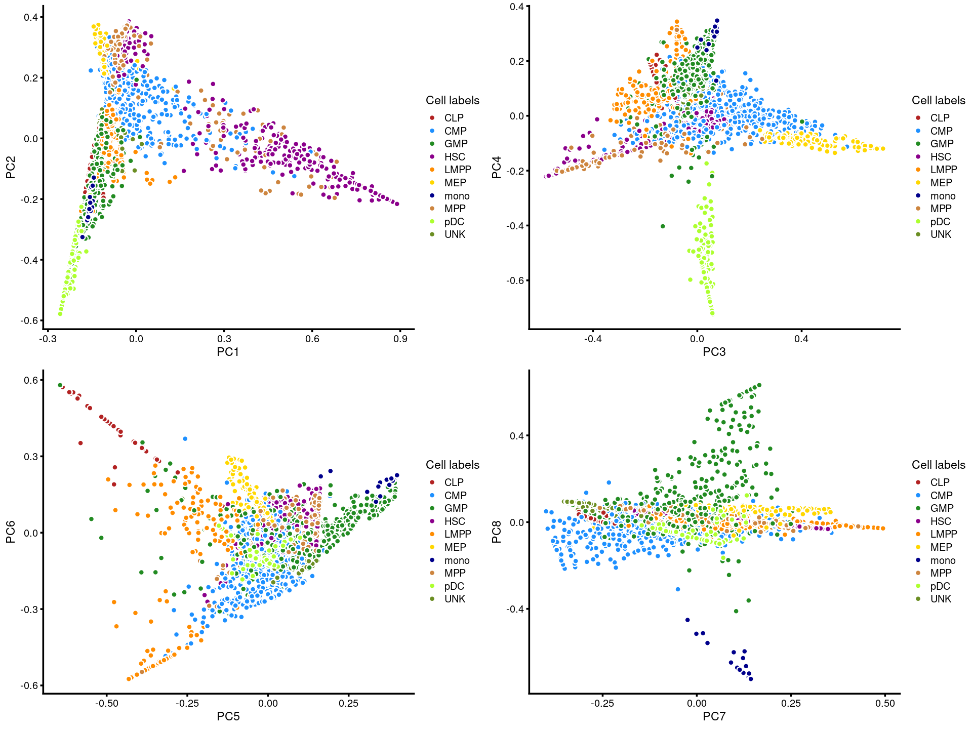
| Version | Author | Date |
|---|---|---|
| fb6a121 | kevinlkx | 2020-11-06 |
k = 13
Load the \(k = 13\) Poisson NMF fit.
out.dir <- "/project2/mstephens/kevinluo/scATACseq-topics/output/Buenrostro_2018/binarized/"
fit <- readRDS(file.path(out.dir, "/fit-Buenrostro2018-binarized-scd-ex-k=13.rds"))$fit
Plot PCs of the topic proportions.
p.pca1.1 <- pca_plot(poisson2multinom(fit),pcs = 1:2,fill = "none")
p.pca1.2 <- pca_plot(poisson2multinom(fit),pcs = 3:4,fill = "none")
p.pca1.3 <- pca_plot(poisson2multinom(fit),pcs = 5:6,fill = "none")
p.pca1.4 <- pca_plot(poisson2multinom(fit),pcs = 7:8,fill = "none")

plot_grid(p.pca1.1,p.pca1.2,p.pca1.3,p.pca1.4)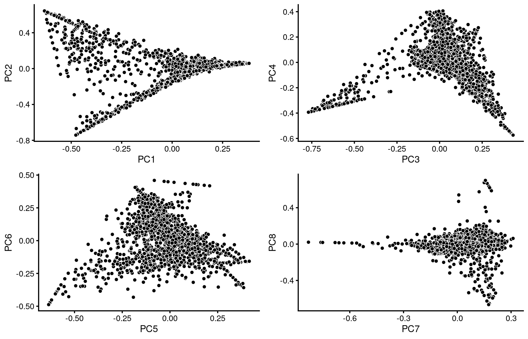
| Version | Author | Date |
|---|---|---|
| fb6a121 | kevinlkx | 2020-11-06 |
Some of the structure is more evident from “hexbin” plots showing the density of the points.
breaks <- c(0,1,5,10,100,Inf)
p.pca2.1 <- pca_hexbin_plot(poisson2multinom(fit), pcs = 1:2, breaks = breaks) + guides(fill = "none")
p.pca2.2 <- pca_hexbin_plot(poisson2multinom(fit), pcs = 3:4, breaks = breaks) + guides(fill = "none")
p.pca2.3 <- pca_hexbin_plot(poisson2multinom(fit), pcs = 5:6, breaks = breaks) + guides(fill = "none")
p.pca2.4 <- pca_hexbin_plot(poisson2multinom(fit), pcs = 7:8, breaks = breaks) + guides(fill = "none")

plot_grid(p.pca2.1,p.pca2.2,p.pca2.3,p.pca2.4)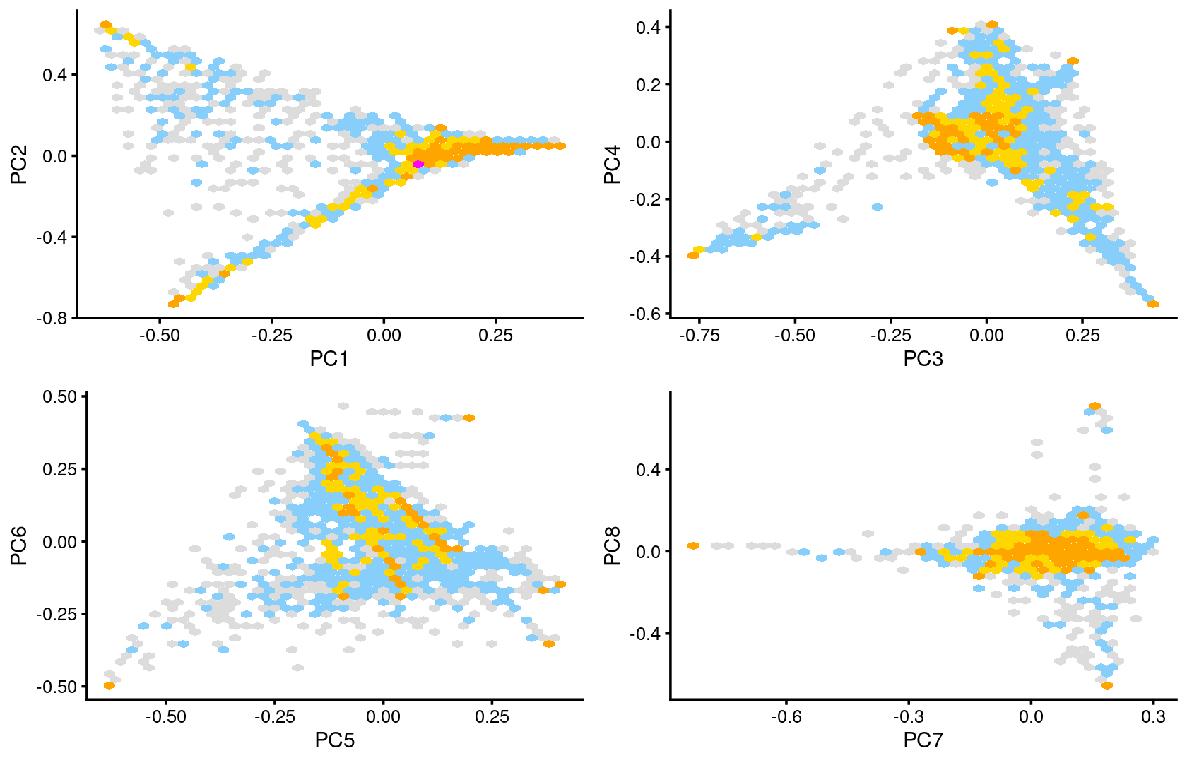
| Version | Author | Date |
|---|---|---|
| fb6a121 | kevinlkx | 2020-11-06 |
Next, we layer the cell labels onto the PC plots.
p.pca3.1 <- labeled_pca_plot(fit,1:2,samples$label,font_size = 7,
                       legend_label = "Cell labels")
p.pca3.2 <- labeled_pca_plot(fit,3:4,samples$label,font_size = 7,
                       legend_label = "Cell labels")
p.pca3.3 <- labeled_pca_plot(fit,5:6,samples$label,font_size = 7,
                       legend_label = "Cell labels")
p.pca3.4 <- labeled_pca_plot(fit,7:8,samples$label,font_size = 7,
                       legend_label = "Cell labels")

plot_grid(p.pca3.1,p.pca3.2,p.pca3.3,p.pca3.4)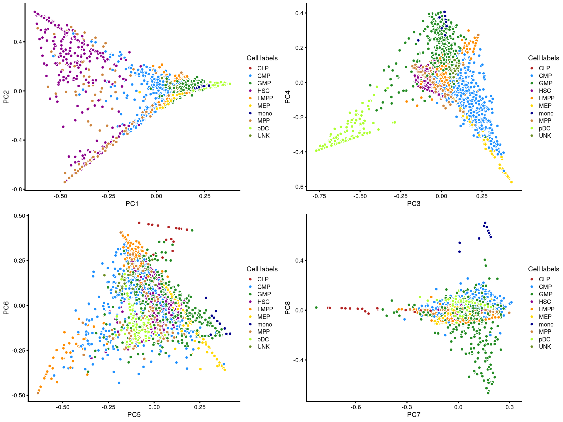
| Version | Author | Date |
|---|---|---|
| fb6a121 | kevinlkx | 2020-11-06 |
k = 14
Load the \(k = 14\) Poisson NMF fit.
out.dir <- "/project2/mstephens/kevinluo/scATACseq-topics/output/Buenrostro_2018/binarized/"
fit <- readRDS(file.path(out.dir, "/fit-Buenrostro2018-binarized-scd-ex-k=14.rds"))$fit
Plot PCs of the topic proportions.
p.pca1.1 <- pca_plot(poisson2multinom(fit),pcs = 1:2,fill = "none")
p.pca1.2 <- pca_plot(poisson2multinom(fit),pcs = 3:4,fill = "none")
p.pca1.3 <- pca_plot(poisson2multinom(fit),pcs = 5:6,fill = "none")
p.pca1.4 <- pca_plot(poisson2multinom(fit),pcs = 7:8,fill = "none")

plot_grid(p.pca1.1,p.pca1.2,p.pca1.3,p.pca1.4)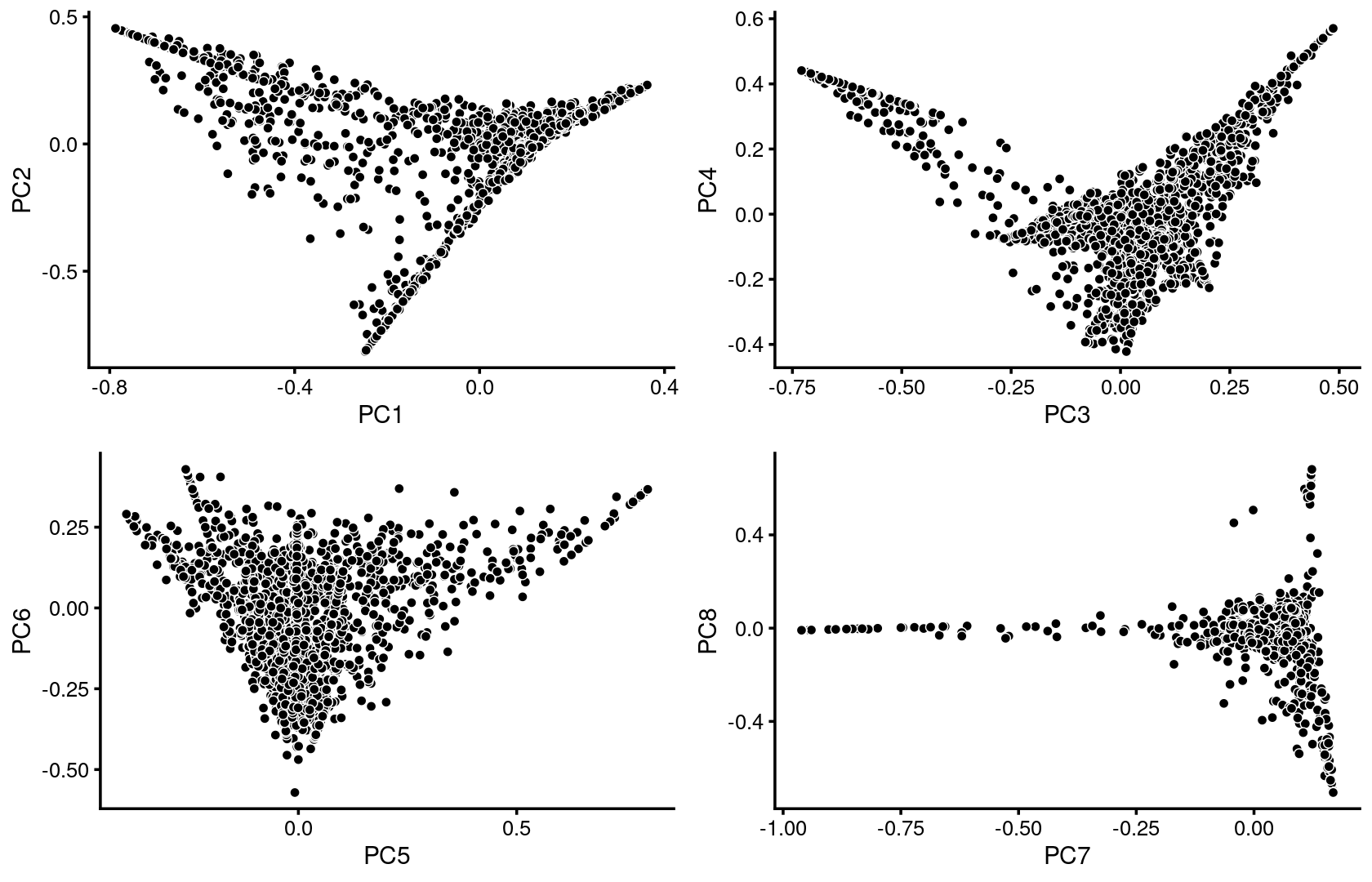
| Version | Author | Date |
|---|---|---|
| fb6a121 | kevinlkx | 2020-11-06 |
Some of the structure is more evident from “hexbin” plots showing the density of the points.
breaks <- c(0,1,5,10,100,Inf)
p.pca2.1 <- pca_hexbin_plot(poisson2multinom(fit), pcs = 1:2, breaks = breaks) + guides(fill = "none")
p.pca2.2 <- pca_hexbin_plot(poisson2multinom(fit), pcs = 3:4, breaks = breaks) + guides(fill = "none")
p.pca2.3 <- pca_hexbin_plot(poisson2multinom(fit), pcs = 5:6, breaks = breaks) + guides(fill = "none")
p.pca2.4 <- pca_hexbin_plot(poisson2multinom(fit), pcs = 7:8, breaks = breaks) + guides(fill = "none")

plot_grid(p.pca2.1,p.pca2.2,p.pca2.3,p.pca2.4)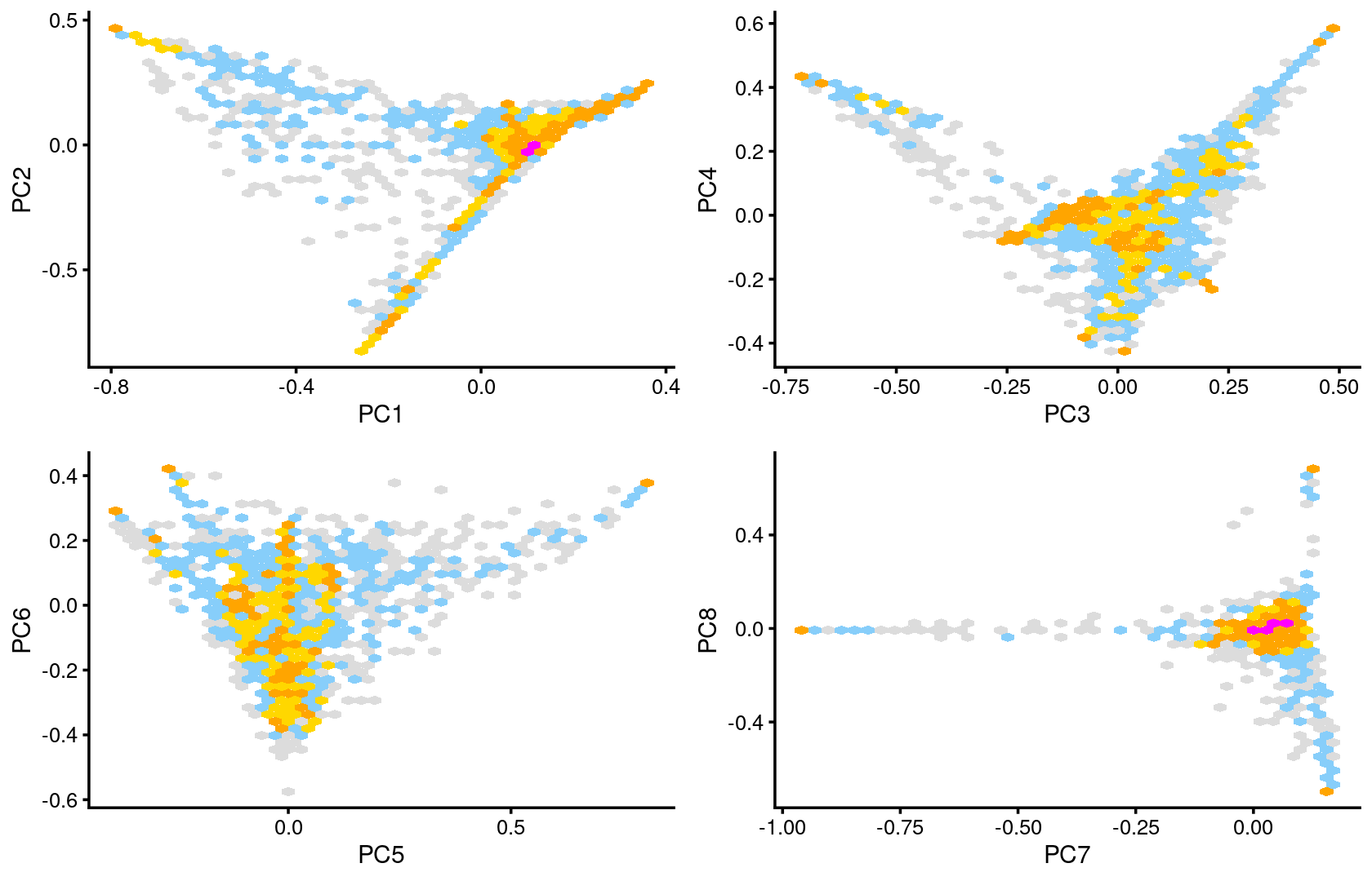
| Version | Author | Date |
|---|---|---|
| fb6a121 | kevinlkx | 2020-11-06 |
Next, we layer the cell labels onto the PC plots.
p.pca3.1 <- labeled_pca_plot(fit,1:2,samples$label,font_size = 7,
                       legend_label = "Cell labels")
p.pca3.2 <- labeled_pca_plot(fit,3:4,samples$label,font_size = 7,
                       legend_label = "Cell labels")
p.pca3.3 <- labeled_pca_plot(fit,5:6,samples$label,font_size = 7,
                       legend_label = "Cell labels")
p.pca3.4 <- labeled_pca_plot(fit,7:8,samples$label,font_size = 7,
                       legend_label = "Cell labels")

plot_grid(p.pca3.1,p.pca3.2,p.pca3.3,p.pca3.4)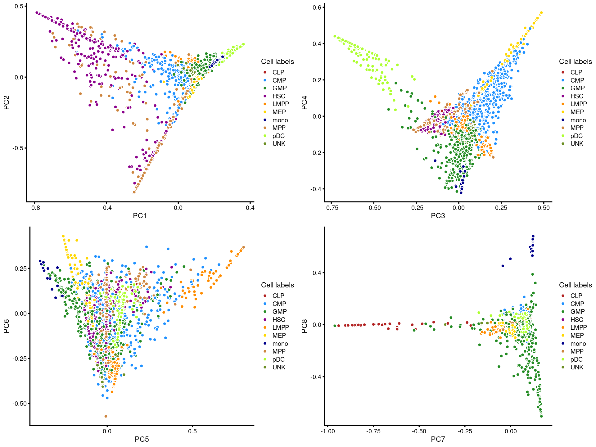
| Version | Author | Date |
|---|---|---|
| fb6a121 | kevinlkx | 2020-11-06 |
k = 15
Load the \(k = 15\) Poisson NMF fit.
out.dir <- "/project2/mstephens/kevinluo/scATACseq-topics/output/Buenrostro_2018/binarized/"
fit <- readRDS(file.path(out.dir, "/fit-Buenrostro2018-binarized-scd-ex-k=15.rds"))$fit
Plot PCs of the topic proportions.
p.pca1.1 <- pca_plot(poisson2multinom(fit),pcs = 1:2,fill = "none")
p.pca1.2 <- pca_plot(poisson2multinom(fit),pcs = 3:4,fill = "none")
p.pca1.3 <- pca_plot(poisson2multinom(fit),pcs = 5:6,fill = "none")
p.pca1.4 <- pca_plot(poisson2multinom(fit),pcs = 7:8,fill = "none")

plot_grid(p.pca1.1,p.pca1.2,p.pca1.3,p.pca1.4)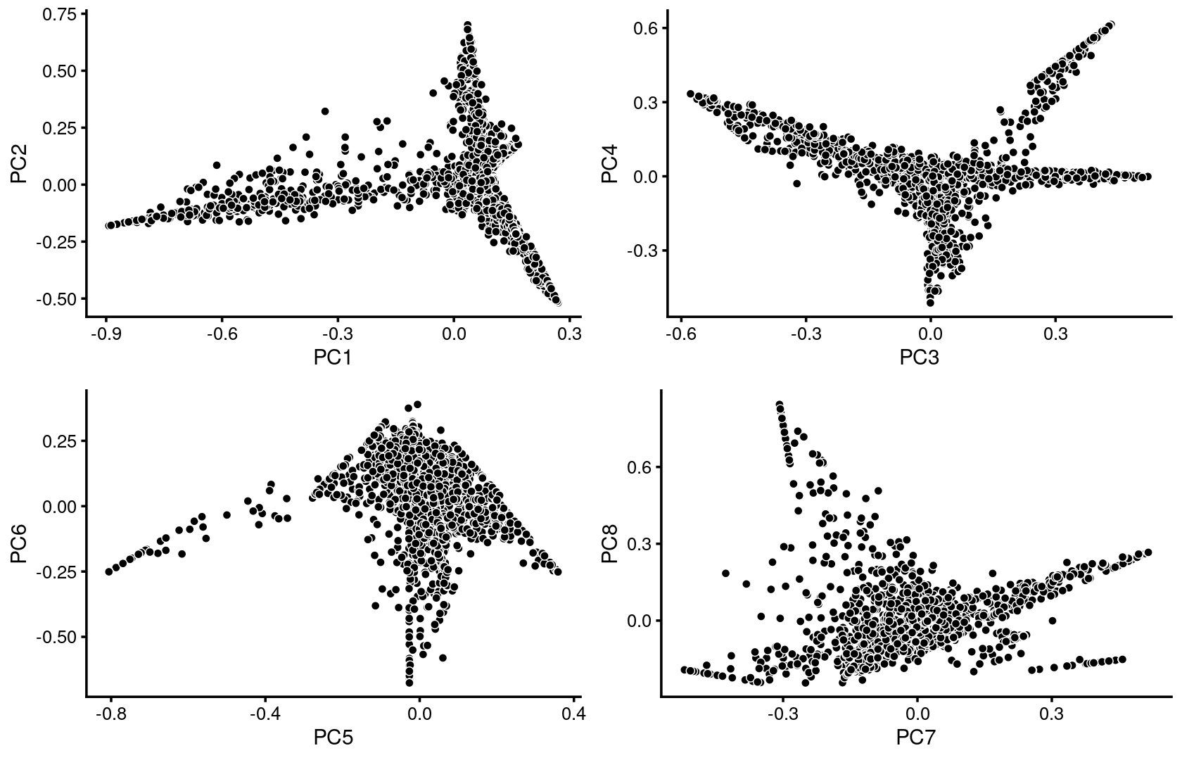
| Version | Author | Date |
|---|---|---|
| fb6a121 | kevinlkx | 2020-11-06 |
Some of the structure is more evident from “hexbin” plots showing the density of the points.
breaks <- c(0,1,5,10,100,Inf)
p.pca2.1 <- pca_hexbin_plot(poisson2multinom(fit), pcs = 1:2, breaks = breaks) + guides(fill = "none")
p.pca2.2 <- pca_hexbin_plot(poisson2multinom(fit), pcs = 3:4, breaks = breaks) + guides(fill = "none")
p.pca2.3 <- pca_hexbin_plot(poisson2multinom(fit), pcs = 5:6, breaks = breaks) + guides(fill = "none")
p.pca2.4 <- pca_hexbin_plot(poisson2multinom(fit), pcs = 7:8, breaks = breaks) + guides(fill = "none")

plot_grid(p.pca2.1,p.pca2.2,p.pca2.3,p.pca2.4)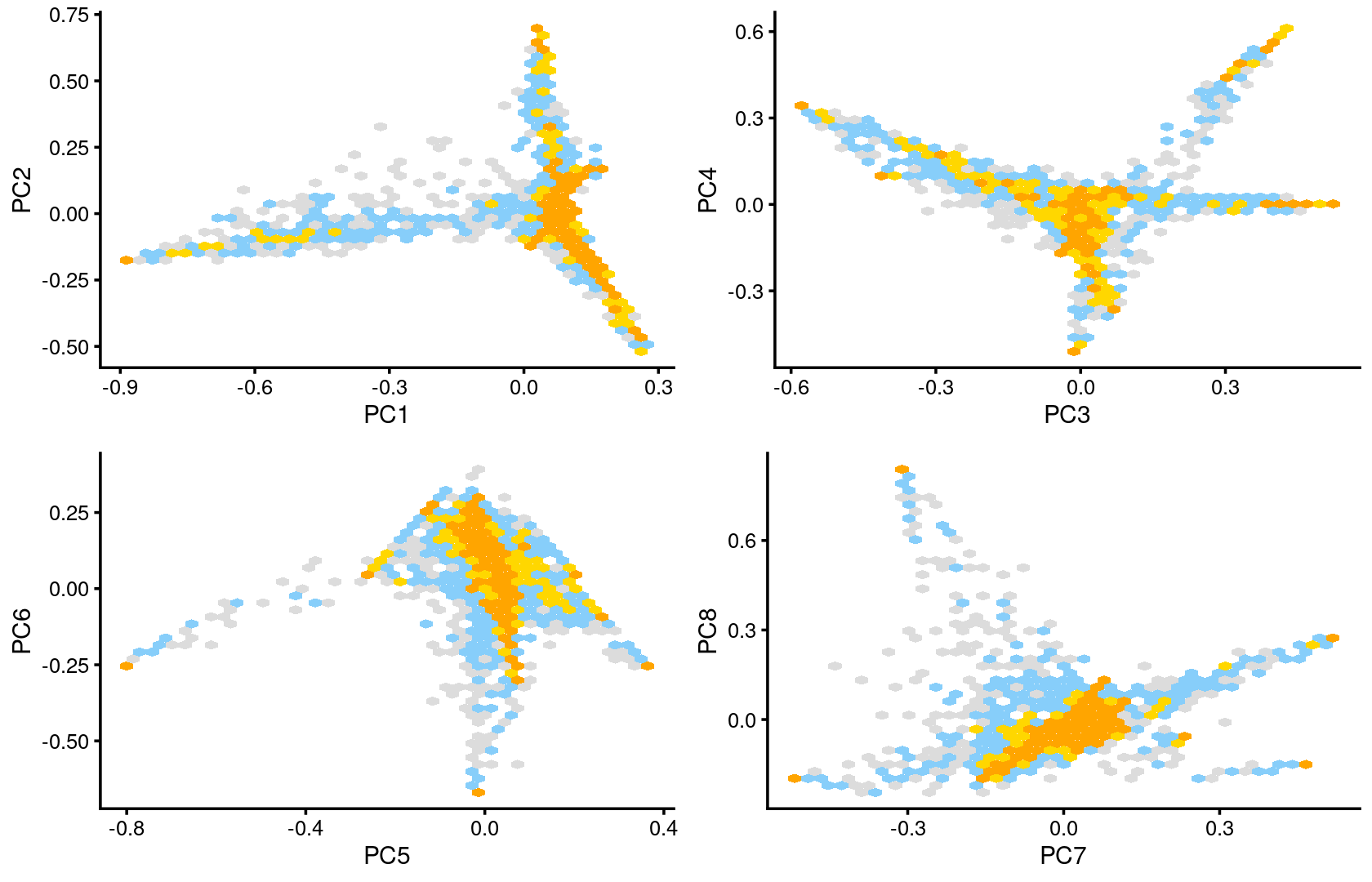
| Version | Author | Date |
|---|---|---|
| fb6a121 | kevinlkx | 2020-11-06 |
Next, we layer the cell labels onto the PC plots.
p.pca3.1 <- labeled_pca_plot(fit,1:2,samples$label,font_size = 7,
                       legend_label = "Cell labels")
p.pca3.2 <- labeled_pca_plot(fit,3:4,samples$label,font_size = 7,
                       legend_label = "Cell labels")
p.pca3.3 <- labeled_pca_plot(fit,5:6,samples$label,font_size = 7,
                       legend_label = "Cell labels")
p.pca3.4 <- labeled_pca_plot(fit,7:8,samples$label,font_size = 7,
                       legend_label = "Cell labels")

plot_grid(p.pca3.1,p.pca3.2,p.pca3.3,p.pca3.4)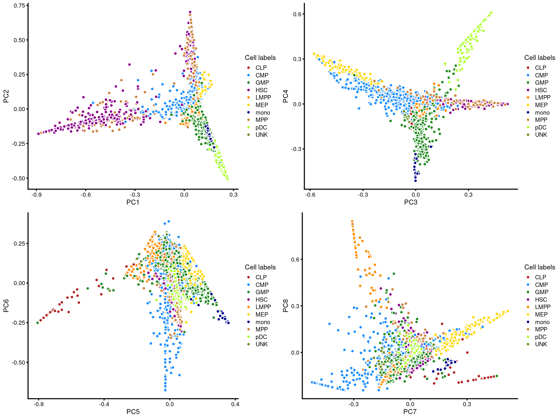
| Version | Author | Date |
|---|---|---|
| fb6a121 | kevinlkx | 2020-11-06 |
sessionInfo()
# R version 3.6.1 (2019-07-05)
# Platform: x86_64-pc-linux-gnu (64-bit)
# Running under: Scientific Linux 7.4 (Nitrogen)
#
# Matrix products: default
# BLAS/LAPACK: /software/openblas-0.2.19-el7-x86_64/lib/libopenblas_haswellp-r0.2.19.so
#
# locale:
#  [1] LC_CTYPE=en_US.UTF-8       LC_NUMERIC=C
#  [3] LC_TIME=en_US.UTF-8        LC_COLLATE=en_US.UTF-8
#  [5] LC_MONETARY=en_US.UTF-8    LC_MESSAGES=en_US.UTF-8
#  [7] LC_PAPER=en_US.UTF-8       LC_NAME=C
#  [9] LC_ADDRESS=C               LC_TELEPHONE=C
# [11] LC_MEASUREMENT=en_US.UTF-8 LC_IDENTIFICATION=C
#
# attached base packages:
# [1] stats     graphics  grDevices utils     datasets  methods   base
#
# other attached packages:
# [1] fastTopics_0.3-180 cowplot_1.0.0      ggplot2_3.3.2      Matrix_1.2-18
# [5] workflowr_1.6.2
#
# loaded via a namespace (and not attached):
#  [1] ggrepel_0.8.2      Rcpp_1.0.5         lattice_0.20-38    tidyr_1.1.0
#  [5] prettyunits_1.1.1  assertthat_0.2.1   rprojroot_1.3-2    digest_0.6.27
#  [9] R6_2.5.0           backports_1.1.10   MatrixModels_0.4-1 evaluate_0.14
# [13] coda_0.19-3        httr_1.4.1         pillar_1.4.6       rlang_0.4.8
# [17] progress_1.2.2     lazyeval_0.2.2     data.table_1.12.8  irlba_2.3.3
# [21] SparseM_1.77       hexbin_1.28.1      whisker_0.4        rmarkdown_2.1
# [25] labeling_0.4.2     Rtsne_0.15         stringr_1.4.0      htmlwidgets_1.5.1
# [29] munsell_0.5.0      compiler_3.6.1     httpuv_1.5.3.1     xfun_0.14
# [33] pkgconfig_2.0.3    mcmc_0.9-7         htmltools_0.4.0    tidyselect_1.1.0
# [37] tibble_3.0.4       quadprog_1.5-7     viridisLite_0.3.0  crayon_1.3.4
# [41] dplyr_0.8.5        withr_2.3.0        later_1.0.0        MASS_7.3-51.6
# [45] grid_3.6.1         jsonlite_1.6       gtable_0.3.0       lifecycle_0.2.0
# [49] git2r_0.27.1       magrittr_1.5       scales_1.1.1       RcppParallel_4.4.3
# [53] stringi_1.4.6      farver_2.0.3       fs_1.3.1           promises_1.1.0
# [57] ellipsis_0.3.1     vctrs_0.3.4        tools_3.6.1        glue_1.4.2
# [61] purrr_0.3.4        hms_0.5.3          yaml_2.2.0         colorspace_1.4-1
# [65] plotly_4.9.0       knitr_1.28         quantreg_5.41      MCMCpack_1.4-4