Topic modeling analysis of Buenrostro et al (2018) data with k = 10 topics
Peter Carbonetto
Last updated: 2022-07-13
Checks: 7 0
Knit directory: scATACseq-topics/
This reproducible R Markdown analysis was created with workflowr (version 1.7.0). The Checks tab describes the reproducibility checks that were applied when the results were created. The Past versions tab lists the development history.
Great! Since the R Markdown file has been committed to the Git repository, you know the exact version of the code that produced these results.
Great job! The global environment was empty. Objects defined in the global environment can affect the analysis in your R Markdown file in unknown ways. For reproduciblity it’s best to always run the code in an empty environment.
The command set.seed(20200729) was run prior to running
the code in the R Markdown file. Setting a seed ensures that any results
that rely on randomness, e.g. subsampling or permutations, are
reproducible.
Great job! Recording the operating system, R version, and package versions is critical for reproducibility.
Nice! There were no cached chunks for this analysis, so you can be confident that you successfully produced the results during this run.
Great job! Using relative paths to the files within your workflowr project makes it easier to run your code on other machines.
Great! You are using Git for version control. Tracking code development and connecting the code version to the results is critical for reproducibility.
The results in this page were generated with repository version dcc8027. See the Past versions tab to see a history of the changes made to the R Markdown and HTML files.
Note that you need to be careful to ensure that all relevant files for
the analysis have been committed to Git prior to generating the results
(you can use wflow_publish or
wflow_git_commit). workflowr only checks the R Markdown
file, but you know if there are other scripts or data files that it
depends on. Below is the status of the Git repository when the results
were generated:
Ignored files:
    Ignored:    .DS_Store
    Ignored:    data/.DS_Store
    Ignored:    data/Buenrostro_2018/
    Ignored:    output/Buenrostro_2018/binarized/filtered_peaks/de-buenrostro2018-k=10-noshrink.RData
    Ignored:    output/Buenrostro_2018/binarized/filtered_peaks/fit-Buenrostro2018-binarized-filtered-scd-ex-k=10.rds
    Ignored:    output/Buenrostro_2018/binarized/filtered_peaks/fit-Buenrostro2018-binarized-filtered-scd-ex-k=8.rds

Untracked files:
    Untracked:  analysis/fit-Buenrostro2018-binarized-scd-ex-k=10.rds
    Untracked:  data/Buenrostro_2018_binarized.RData
    Untracked:  output/Buenrostro_2018/binarized/filtered_peaks/Buenrostro_2018_binarized_filtered.RData
    Untracked:  plots/
    Untracked:  scripts/fit-buenrostro-2018-k=8.rds
    Untracked:  scripts/structure_plot_buenrostro2018.png

Unstaged changes:
    Modified:   analysis/temp.R
Note that any generated files, e.g. HTML, png, CSS, etc., are not included in this status report because it is ok for generated content to have uncommitted changes.
These are the previous versions of the repository in which changes were
made to the R Markdown (analysis/buenrostro2018_k10.Rmd)
and HTML (docs/buenrostro2018_k10.html) files. If you’ve
configured a remote Git repository (see ?wflow_git_remote),
click on the hyperlinks in the table below to view the files as they
were in that past version.
| File | Version | Author | Date | Message |
|---|---|---|---|---|
| Rmd | dcc8027 | Peter Carbonetto | 2022-07-13 | workflowr::wflow_publish("analysis/buenrostro2018_k10.Rmd", verbose = TRUE) |
| Rmd | 287aee7 | Peter Carbonetto | 2022-07-13 | Added some text to the buenrostro2018_k10 analysis and revised the structure plot a bit. |
| Rmd | ebcdcc4 | Peter Carbonetto | 2022-07-12 | In temp.R I have a tile plot I am mostly happy with. |
| html | 8fac509 | Peter Carbonetto | 2022-07-11 | Created exploratory script temp.R. |
| html | 0493e2f | Peter Carbonetto | 2022-05-10 | Added volcano plots to buenrostro2018_k10 analysis. |
| Rmd | a49e37e | Peter Carbonetto | 2022-05-10 | workflowr::wflow_publish("analysis/buenrostro2018_k10.Rmd", verbose = TRUE) |
| html | 63d0c5c | Peter Carbonetto | 2022-05-03 | Improved the structure plot in the buenrostro2018_k10 analysis. |
| Rmd | 2fc232b | Peter Carbonetto | 2022-05-03 | workflowr::wflow_publish("buenrostro2018_k10.Rmd", verbose = TRUE) |
| Rmd | 7853353 | Peter Carbonetto | 2022-05-03 | workflowr::wflow_rename("buenrostro2018_k8.Rmd", "buenrostro2018_k10.Rmd") |
| html | 7853353 | Peter Carbonetto | 2022-05-03 | workflowr::wflow_rename("buenrostro2018_k8.Rmd", "buenrostro2018_k10.Rmd") |
Here we summarize and interpret the results from the topic modeling analysis of the Buenrostro et al (2018) data, with \(k = 10\) topics.
Load the packages used in the analysis below.
library(Matrix)
library(fastTopics)
library(ggplot2)
library(cowplot)
Load the count data (see here for details on these data and how they were prepared).
load("data/Buenrostro_2018/processed_data/Buenrostro_2018_binarized.RData")Next we load the \(k = 10\) multinomial topic model fit to these data, the results of the GoM DE analysis using this topic model, and the results of the HOMER motif enrichment analysis using the p-values from the GoM DE analysis:
fit <- readRDS(
  file.path("output/Buenrostro_2018/binarized/filtered_peaks",
            "fit-Buenrostro2018-binarized-filtered-scd-ex-k=10.rds"))$fit
fit <- poisson2multinom(fit)
load(file.path("output/Buenrostro_2018/binarized/filtered_peaks",
               "de-buenrostro2018-k=10-noshrink.RData"))
homer <- readRDS(file.path("output/Buenrostro_2018/binarized/filtered_peaks",
                           "homer-buenrostro2018-k=10-noshrink.rds"))
Visualize the structure identified in the FACS cell populations using a Structure plot:
set.seed(1)
celltypes <- factor(samples$label,
                    c("pDC","CLP","LMPP","HSC","MPP","CMP","MEP","GMP",
                      "mono","UNK"))
topic_colors <- c("gold","forestgreen","orchid","red","lightgray",
                  "dimgray","orange","dodgerblue","limegreen","mediumblue")
p1 <- structure_plot(fit,grouping = celltypes,n = Inf,gap = 20,
                     perplexity = 70,verbose = FALSE,colors = topic_colors,
                     topics = c(5,10,8,3,4,1,6,7,2,9))
print(p1)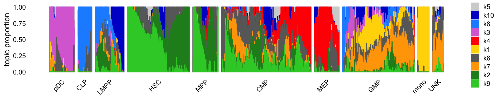
Comparing the topic proportions with the cell labels (provided by FACS), we see that the topics capture chromatin accessibility patterns characteristic of early hematopoietic progenitors (HSC, MPP; topics 2 and 9), and the four different hematopoietic cell lineages: CLPs and LMPPs (topic 8); pDCs (topic 3); monocytes and GMPs (topics 1 and 7); and MEPs (topic 4). Additional topics (topics 5, 6 and 10) may be picking up other factors such as patient-specific batch effects or tissue of origin (bone marrow or blood). Additionally, the split of the HSC/MPP cells into two topics seems to also reflect patient-specific batch effects, which also came up in the PCA analysis in the original paper.
The de_analysis function attempts to quantify
differential accessibility in each of the peaks:
n <- nrow(de$z)
k <- ncol(de$z)
p <- vector("list",k)
names(p) <- colnames(de$z)
for (i in 1:k)
  p[[i]] <- volcano_plot(de,i,labels = rep("",n)) +
    guides(fill = "none")
do.call("plot_grid",c(p,list(nrow = 4,ncol = 3)))
The individual results are not strong, but an enrichment analysis of the peaks might point to interesting patterns among these differentially accessible peaks.
sessionInfo()
# R version 3.6.2 (2019-12-12)
# Platform: x86_64-apple-darwin15.6.0 (64-bit)
# Running under: macOS Catalina 10.15.7
#
# Matrix products: default
# BLAS:   /Library/Frameworks/R.framework/Versions/3.6/Resources/lib/libRblas.0.dylib
# LAPACK: /Library/Frameworks/R.framework/Versions/3.6/Resources/lib/libRlapack.dylib
#
# locale:
# [1] en_US.UTF-8/en_US.UTF-8/en_US.UTF-8/C/en_US.UTF-8/en_US.UTF-8
#
# attached base packages:
# [1] stats     graphics  grDevices utils     datasets  methods   base
#
# other attached packages:
# [1] cowplot_1.0.0      ggplot2_3.3.5      fastTopics_0.6-131 Matrix_1.2-18
# [5] workflowr_1.7.0
#
# loaded via a namespace (and not attached):
#  [1] mcmc_0.9-6         fs_1.5.2           progress_1.2.2     httr_1.4.2
#  [5] rprojroot_1.3-2    tools_3.6.2        backports_1.1.5    bslib_0.3.1
#  [9] utf8_1.1.4         R6_2.4.1           irlba_2.3.3        uwot_0.1.10
# [13] DBI_1.1.0          lazyeval_0.2.2     colorspace_1.4-1   withr_2.5.0
# [17] tidyselect_1.1.1   prettyunits_1.1.1  processx_3.5.2     compiler_3.6.2
# [21] git2r_0.29.0       quantreg_5.54      SparseM_1.78       plotly_4.9.2
# [25] labeling_0.3       sass_0.4.0         scales_1.1.0       SQUAREM_2017.10-1
# [29] quadprog_1.5-8     callr_3.7.0        pbapply_1.5-1      mixsqp_0.3-46
# [33] systemfonts_1.0.2  stringr_1.4.0      digest_0.6.23      rmarkdown_2.11
# [37] MCMCpack_1.4-5     pkgconfig_2.0.3    htmltools_0.5.2    fastmap_1.1.0
# [41] invgamma_1.1       highr_0.8          htmlwidgets_1.5.1  rlang_0.4.11
# [45] rstudioapi_0.13    jquerylib_0.1.4    generics_0.0.2     farver_2.0.1
# [49] jsonlite_1.7.2     dplyr_1.0.7        magrittr_2.0.1     Rcpp_1.0.7
# [53] munsell_0.5.0      fansi_0.4.0        lifecycle_1.0.0    stringi_1.4.3
# [57] whisker_0.4        yaml_2.2.0         MASS_7.3-51.4      Rtsne_0.15
# [61] grid_3.6.2         parallel_3.6.2     promises_1.1.0     ggrepel_0.9.1
# [65] crayon_1.4.1       lattice_0.20-38    hms_1.1.0          knitr_1.37
# [69] ps_1.6.0           pillar_1.6.2       glue_1.4.2         evaluate_0.14
# [73] getPass_0.2-2      data.table_1.12.8  RcppParallel_5.1.5 vctrs_0.3.8
# [77] httpuv_1.5.2       MatrixModels_0.4-1 gtable_0.3.0       purrr_0.3.4
# [81] tidyr_1.1.3        assertthat_0.2.1   ashr_2.2-54        xfun_0.29
# [85] coda_0.19-3        later_1.0.0        ragg_0.3.1         viridisLite_0.3.0
# [89] truncnorm_1.0-8    tibble_3.1.3       ellipsis_0.3.2