Motif analysis using topic modeling and DA results (v2) for Buenrostro et al (2018) scATAC-seq result
Kaixuan Luo
Last updated: 2022-03-09
Checks: 7 0
Knit directory: scATACseq-topics/
This reproducible R Markdown analysis was created with workflowr (version 1.7.0). The Checks tab describes the reproducibility checks that were applied when the results were created. The Past versions tab lists the development history.
Great! Since the R Markdown file has been committed to the Git repository, you know the exact version of the code that produced these results.
Great job! The global environment was empty. Objects defined in the global environment can affect the analysis in your R Markdown file in unknown ways. For reproduciblity it's best to always run the code in an empty environment.
The command set.seed(20200729) was run prior to running the code in the R Markdown file. Setting a seed ensures that any results that rely on randomness, e.g. subsampling or permutations, are reproducible.
Great job! Recording the operating system, R version, and package versions is critical for reproducibility.
Nice! There were no cached chunks for this analysis, so you can be confident that you successfully produced the results during this run.
Great job! Using relative paths to the files within your workflowr project makes it easier to run your code on other machines.
Great! You are using Git for version control. Tracking code development and connecting the code version to the results is critical for reproducibility.
The results in this page were generated with repository version 6baae37. See the Past versions tab to see a history of the changes made to the R Markdown and HTML files.
Note that you need to be careful to ensure that all relevant files for the analysis have been committed to Git prior to generating the results (you can use wflow_publish or wflow_git_commit). workflowr only checks the R Markdown file, but you know if there are other scripts or data files that it depends on. Below is the status of the Git repository when the results were generated:
Ignored files:
    Ignored:    .DS_Store
    Ignored:    .Rhistory
    Ignored:    .Rproj.user/

Untracked files:
    Untracked:  analysis/gene_analysis_Buenrostro2018_v2.Rmd
    Untracked:  analysis/motif_analysis_Buenrostro2018_v2.Rmd
    Untracked:  output/clustering-Cusanovich2018.rds
    Untracked:  paper/

Unstaged changes:
    Modified:   analysis/assess_fits_Buenrostro2018_Chen2019pipeline.Rmd
    Modified:   analysis/clusters_Cusanovich2018_k13.Rmd
    Modified:   analysis/gene_analysis_Buenrostro2018_Chen2019pipeline.Rmd
    Modified:   analysis/gene_analysis_Cusanovich2018.Rmd
    Modified:   analysis/motif_analysis_Buenrostro2018_Chen2019pipeline.Rmd
    Modified:   analysis/motif_analysis_Cusanovich2018.Rmd
    Modified:   analysis/plots_Cusanovich2018.Rmd
    Modified:   scripts/postfit_Buenrostro2018_v2.sh
Note that any generated files, e.g. HTML, png, CSS, etc., are not included in this status report because it is ok for generated content to have uncommitted changes.
These are the previous versions of the repository in which changes were made to the R Markdown (analysis/motif_analysis_Buenrostro2018_k10_v2.Rmd) and HTML (docs/motif_analysis_Buenrostro2018_k10_v2.html) files. If you've configured a remote Git repository (see ?wflow_git_remote), click on the hyperlinks in the table below to view the files as they were in that past version.
| File | Version | Author | Date | Message |
|---|---|---|---|---|
| Rmd | 6baae37 | kevinlkx | 2022-03-09 | corrected a typo of k |
| html | bdd0a99 | kevinlkx | 2022-03-09 | Build site. |
| Rmd | 1b7f106 | kevinlkx | 2022-03-09 | do not show all motif enrichment results |
| html | 38627c5 | kevinlkx | 2022-03-09 | Build site. |
| Rmd | e17fb16 | kevinlkx | 2022-03-09 | switched the order of showing motif enrichment results |
| html | 3551232 | kevinlkx | 2022-03-09 | Build site. |
| Rmd | 6954b87 | kevinlkx | 2022-03-09 | updated motif enrichment results with four different methods |
Here we perform TF motif analysis for the Buenrostro et al (2018) scATAC-seq result inferred from the multinomial topic model with \(k = 10\).
We use binarized data downloaded from original paper.
Load packages and some functions used in this analysis
library(Matrix)
library(fastTopics)
library(dplyr)
library(tidyr)
library(ggplot2)
library(ggrepel)
library(cowplot)
library(plotly)
library(DT)
library(reshape2)
source("code/motif_analysis.R")
source("code/plots.R")
Load data and topic model results
Data downloaded from original paper. Load the binarized data and the \(k = 10\) Poisson NMF fit results
data.dir <- "/project2/mstephens/kevinluo/scATACseq-topics/data/Buenrostro_2018/processed_data/"
load(file.path(data.dir, "Buenrostro_2018_binarized_counts.RData"))
cat(sprintf("%d x %d counts matrix.\n",nrow(counts),ncol(counts)))
# 2953 x 491437 counts matrix.fit.dir <- "/project2/mstephens/kevinluo/scATACseq-topics/output/Buenrostro_2018/binarized/"
fit <- readRDS(file.path(fit.dir, "/fit-Buenrostro2018-binarized-scd-ex-k=10.rds"))$fit
fit <- poisson2multinom(fit)Structure plot
topic_colors <- c("darkorange","limegreen","magenta","gold","skyblue",
                  "darkblue","dodgerblue","darkmagenta","red","olivedrab")

set.seed(1)
# labels <- factor(samples$label, levels = c("HSC", "MPP", "CMP", "GMP", "mono", "MEP", "LMPP", "CLP", "pDC", "UNK"))

labels <- factor(samples$label, c("mono","pDC","MEP","HSC","MPP","CLP",
                                 "LMPP","CMP","GMP","UNK"))
structure_plot(fit,grouping = labels,colors = topic_colors,
               # topics = 1:10,
               gap = 20,perplexity = 50,verbose = FALSE)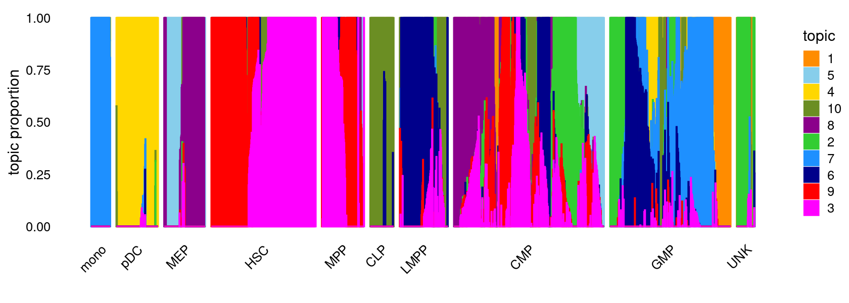
| Version | Author | Date |
|---|---|---|
| 3551232 | kevinlkx | 2022-03-09 |
Motif enrichment analysis using HOMER
- About HOMER motif analysis
- Script for motif enrichment analysis using HOMER
Motif enrichment result using regions with DA p-value < 0.05
Load and compile HOMER results across topics
postfit.dir <- "/project2/mstephens/kevinluo/scATACseq-topics/output/Buenrostro_2018/binarized/postfit_v2"
homer.dir <- paste0(postfit.dir, "/motifanalysis-Buenrostro2018-k=10/HOMER/DA_pval_0.05_regions")
cat(sprintf("Directory of motif analysis result: %s \n", homer.dir))
homer_res_topics <- readRDS(file.path(homer.dir, "/homer_knownResults.rds"))
selected_regions <- readRDS(file.path(homer.dir, "/selected_regions.rds"))

# Compile Homer results (pvalue and ranking) across topics
motif_res <- compile_homer_motif_res(homer_res_topics)
saveRDS(motif_res, paste0(homer.dir, "/homer_motif_enrichment_results.rds"))
cat("compiled homer motif results are saved in", paste0(homer.dir, "/homer_motif_enrichment_results.rds \n"))
# Directory of motif analysis result: /project2/mstephens/kevinluo/scATACseq-topics/output/Buenrostro_2018/binarized/postfit_v2/motifanalysis-Buenrostro2018-k=10/HOMER/DA_pval_0.05_regions
# compiled homer motif results are saved in /project2/mstephens/kevinluo/scATACseq-topics/output/Buenrostro_2018/binarized/postfit_v2/motifanalysis-Buenrostro2018-k=10/HOMER/DA_pval_0.05_regions/homer_motif_enrichment_results.rdsTop 10 motifs for each topic
cat("Number of regions selected for each topic: \n")
print(mapply(nrow, selected_regions[1:(length(selected_regions)-1)]))

colnames_homer <- c("motif_name", "consensus", "P", "log10P", "Padj",  "num_target", "percent_target", "num_bg", "percent_bg")

top_motifs <- data.frame(matrix(nrow=10, ncol = length(homer_res_topics)))
colnames(top_motifs) <- names(homer_res_topics)
for (k in 1:length(homer_res_topics)){
  homer_res <- homer_res_topics[[k]]
  colnames(homer_res) <- colnames_homer
  homer_res <- homer_res %>% separate(motif_name, c("motif", "origin", "database"), "/")
  top_motifs[,k] <- head(homer_res$motif, 10)
}

DT::datatable(data.frame(rank = 1:10, top_motifs), rownames = F, caption = "Top 10 motifs enriched in each topic.")
# Number of regions selected for each topic:
# k1 k2 k3 k4 k5 k6 k7 k8 k9 k10
# 40 19 1322 3223 245 73 1385 1882 252 790Heatmap of motif enrichment -log10(p-value).
create_motif_enrichment_heatmap(motif_res, enrichment = "-log10(p-value)",
                                cluster_motifs = TRUE, cluster_topics = TRUE, motif_filter = 10, horizontal = FALSE,
                                enrichment_range = c(0,100), method_cluster = "average", font.size.motifs = 4, font.size.topics = 9)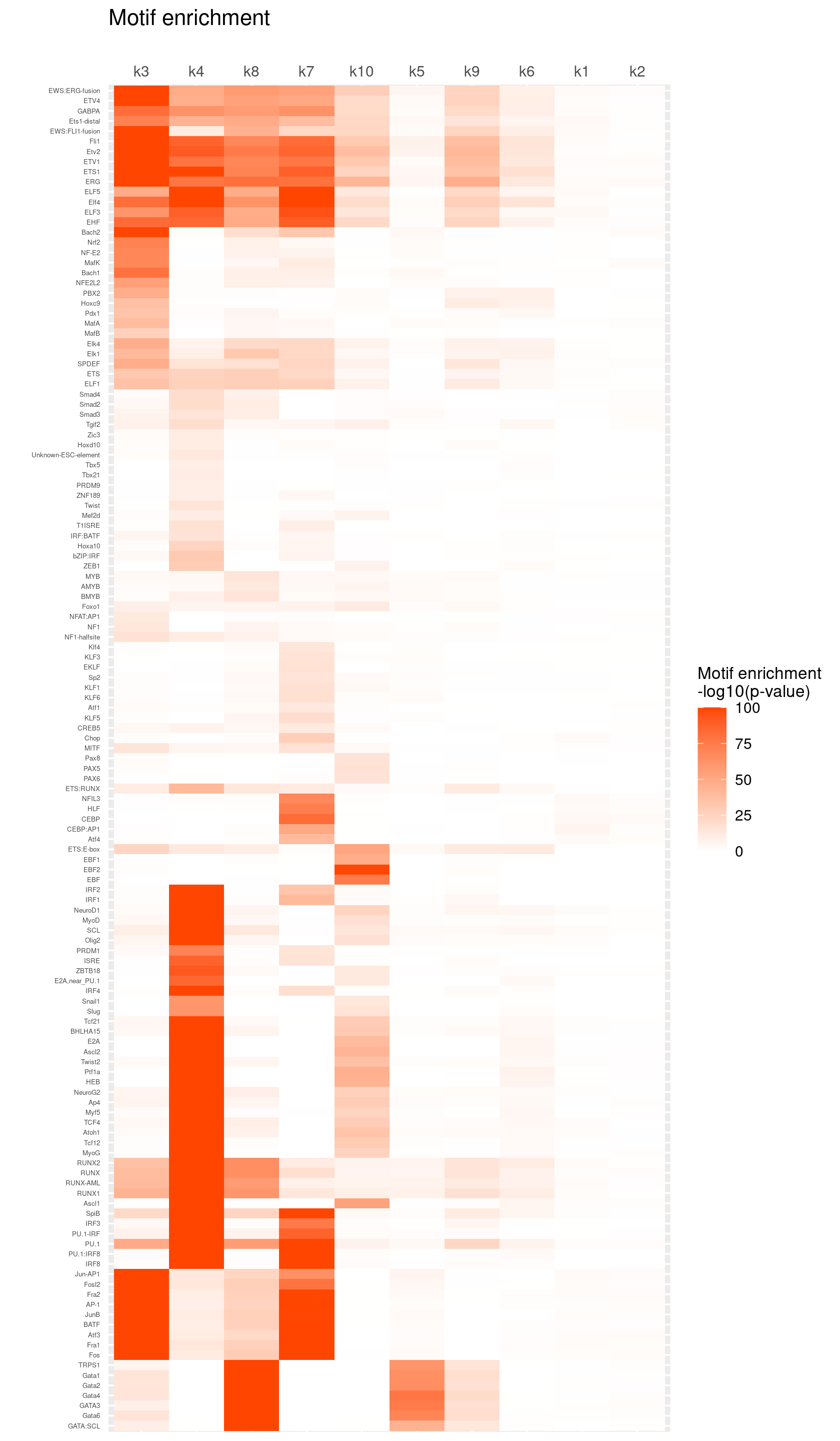
| Version | Author | Date |
|---|---|---|
| 3551232 | kevinlkx | 2022-03-09 |
# 133 out of 439 motifs included the heatmapTop enriched motifs
plots <- vector("list", ncol(motif_res$mlog10P))
names(plots) <- colnames(motif_res$mlog10P)

for( i in 1:length(plots)){
  plots[[i]] <- create_motif_enrichment_ranking_plot(motif_res, k = i,
                                                     max.overlaps = 20, subsample = FALSE)
}

do.call(plot_grid,plots)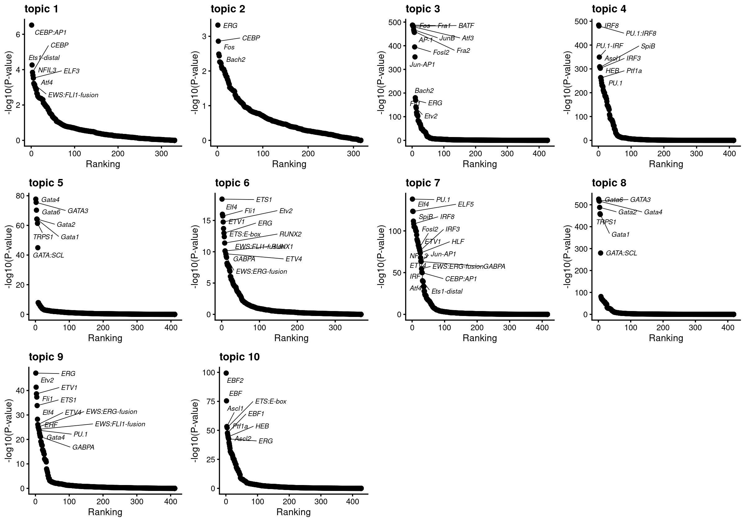
Motif enrichment result using regions with DA p-value < 0.1
Load and compile HOMER results across topics
postfit.dir <- "/project2/mstephens/kevinluo/scATACseq-topics/output/Buenrostro_2018/binarized/postfit_v2"
homer.dir <- paste0(postfit.dir, "/motifanalysis-Buenrostro2018-k=10/HOMER/DA_pval_0.1_regions")
cat(sprintf("Directory of motif analysis result: %s \n", homer.dir))
homer_res_topics <- readRDS(file.path(homer.dir, "/homer_knownResults.rds"))
selected_regions <- readRDS(file.path(homer.dir, "/selected_regions.rds"))

# Compile Homer results (pvalue and ranking) across topics
motif_res <- compile_homer_motif_res(homer_res_topics)
saveRDS(motif_res, paste0(homer.dir, "/homer_motif_enrichment_results.rds"))
cat("compiled homer motif results are saved in", paste0(homer.dir, "/homer_motif_enrichment_results.rds \n"))
# Directory of motif analysis result: /project2/mstephens/kevinluo/scATACseq-topics/output/Buenrostro_2018/binarized/postfit_v2/motifanalysis-Buenrostro2018-k=10/HOMER/DA_pval_0.1_regions
# compiled homer motif results are saved in /project2/mstephens/kevinluo/scATACseq-topics/output/Buenrostro_2018/binarized/postfit_v2/motifanalysis-Buenrostro2018-k=10/HOMER/DA_pval_0.1_regions/homer_motif_enrichment_results.rdsTop 10 motifs for each topic
cat("Number of regions selected for each topic: \n")
print(mapply(nrow, selected_regions[1:(length(selected_regions)-1)]))

colnames_homer <- c("motif_name", "consensus", "P", "log10P", "Padj",  "num_target", "percent_target", "num_bg", "percent_bg")

top_motifs <- data.frame(matrix(nrow=10, ncol = length(homer_res_topics)))
colnames(top_motifs) <- names(homer_res_topics)
for (k in 1:length(homer_res_topics)){
  homer_res <- homer_res_topics[[k]]
  colnames(homer_res) <- colnames_homer
  homer_res <- homer_res %>% separate(motif_name, c("motif", "origin", "database"), "/")
  top_motifs[,k] <- head(homer_res$motif, 10)
}

DT::datatable(data.frame(rank = 1:10, top_motifs), rownames = F, caption = "Top 10 motifs enriched in each topic.")
# Number of regions selected for each topic:
# k1 k2 k3 k4 k5 k6 k7 k8 k9 k10
# 163 45 1793 4250 416 125 2091 2772 418 1191Heatmap of motif enrichment -log10(p-value).
create_motif_enrichment_heatmap(motif_res, enrichment = "-log10(p-value)",
                                cluster_motifs = TRUE, cluster_topics = TRUE, motif_filter = 10, horizontal = FALSE,
                                enrichment_range = c(0,100), method_cluster = "average", font.size.motifs = 4, font.size.topics = 9)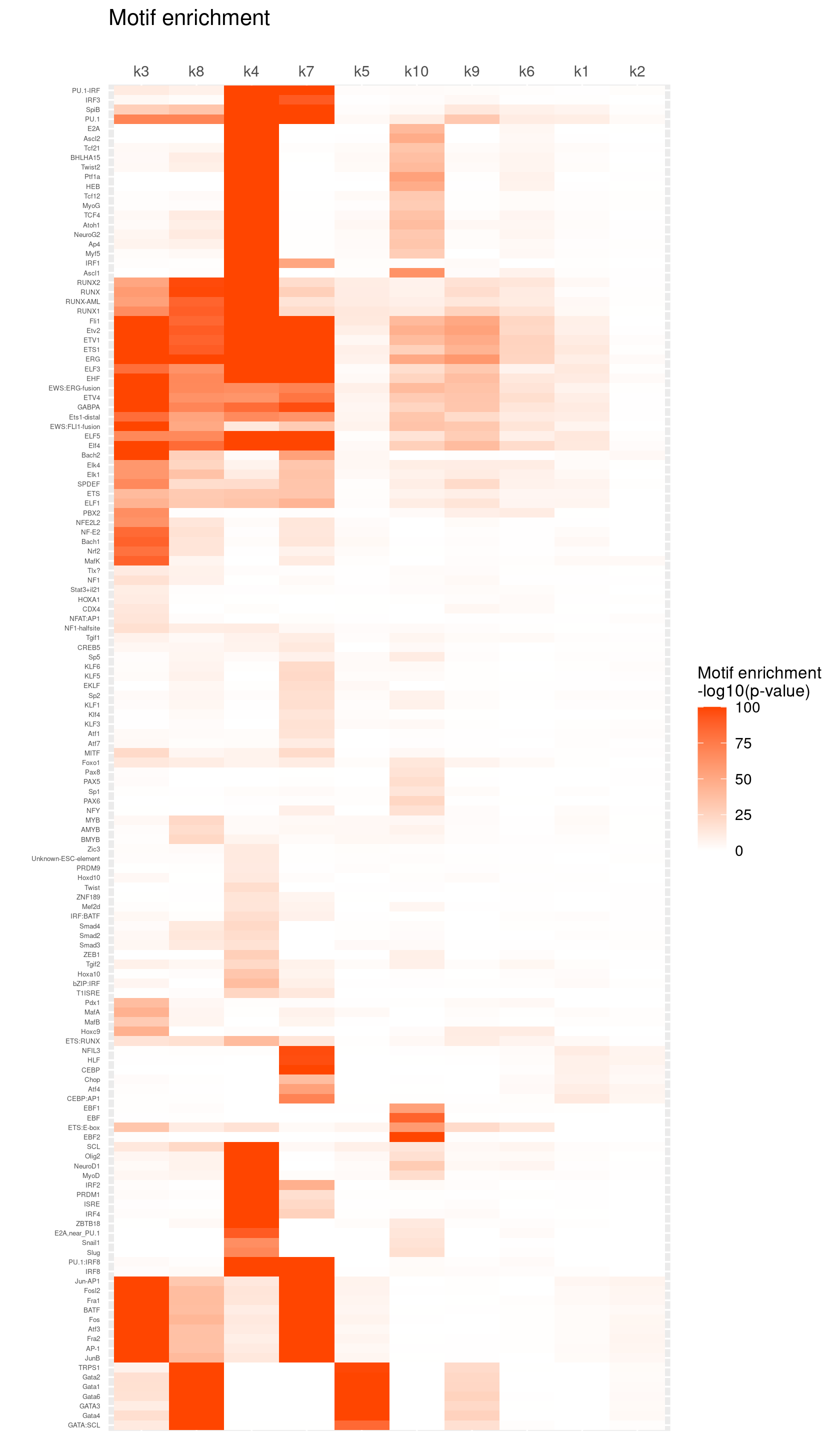
| Version | Author | Date |
|---|---|---|
| 3551232 | kevinlkx | 2022-03-09 |
# 140 out of 439 motifs included the heatmapTop enriched motifs
plots <- vector("list", ncol(motif_res$mlog10P))
names(plots) <- colnames(motif_res$mlog10P)

for( i in 1:length(plots)){
  plots[[i]] <- create_motif_enrichment_ranking_plot(motif_res, k = i,
                                                     max.overlaps = 20, subsample = FALSE)
}

do.call(plot_grid,plots)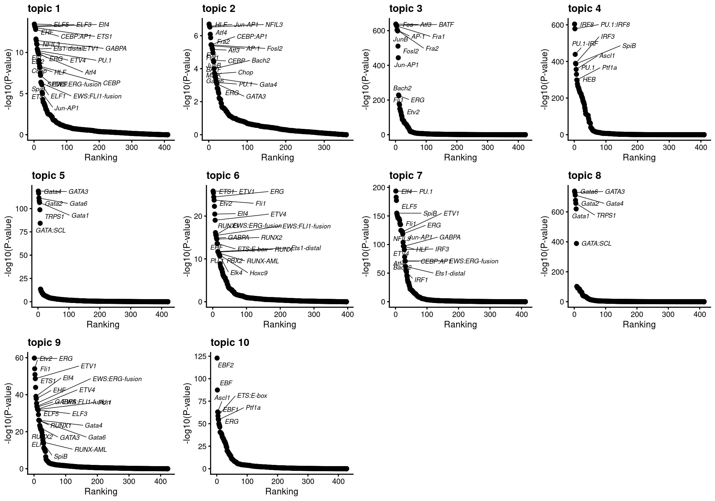
Motif enrichment result using top 1% regions with largest logFC
Load and compile HOMER results across topics
postfit.dir <- "/project2/mstephens/kevinluo/scATACseq-topics/output/Buenrostro_2018/binarized/postfit_v2"
homer.dir <- paste0(postfit.dir, "/motifanalysis-Buenrostro2018-k=10/HOMER/DA_top1percent_regions")
cat(sprintf("Directory of motif analysis result: %s \n", homer.dir))
homer_res_topics <- readRDS(file.path(homer.dir, "/homer_knownResults.rds"))
selected_regions <- readRDS(file.path(homer.dir, "/selected_regions.rds"))

# Compile Homer results (pvalue and ranking) across topics
motif_res <- compile_homer_motif_res(homer_res_topics)
saveRDS(motif_res, paste0(homer.dir, "/homer_motif_enrichment_results.rds"))
cat("compiled homer motif results are saved in", paste0(homer.dir, "/homer_motif_enrichment_results.rds \n"))
# Directory of motif analysis result: /project2/mstephens/kevinluo/scATACseq-topics/output/Buenrostro_2018/binarized/postfit_v2/motifanalysis-Buenrostro2018-k=10/HOMER/DA_top1percent_regions
# compiled homer motif results are saved in /project2/mstephens/kevinluo/scATACseq-topics/output/Buenrostro_2018/binarized/postfit_v2/motifanalysis-Buenrostro2018-k=10/HOMER/DA_top1percent_regions/homer_motif_enrichment_results.rdsTop 10 motifs for each topic
cat("Number of regions selected for each topic: \n")
print(mapply(nrow, selected_regions[1:(length(selected_regions)-1)]))

colnames_homer <- c("motif_name", "consensus", "P", "log10P", "Padj",  "num_target", "percent_target", "num_bg", "percent_bg")

top_motifs <- data.frame(matrix(nrow=10, ncol = length(homer_res_topics)))
colnames(top_motifs) <- names(homer_res_topics)
for (k in 1:length(homer_res_topics)){
  homer_res <- homer_res_topics[[k]]
  colnames(homer_res) <- colnames_homer
  homer_res <- homer_res %>% separate(motif_name, c("motif", "origin", "database"), "/")
  top_motifs[,k] <- head(homer_res$motif, 10)
}

DT::datatable(data.frame(rank = 1:10, top_motifs), rownames = F, caption = "Top 10 motifs enriched in each topic.")
# Number of regions selected for each topic:
# k1 k2 k3 k4 k5 k6 k7 k8 k9 k10
# 4656 4656 4656 4656 4656 4656 4656 4656 4656 4656Heatmap of motif enrichment -log10(p-value).
create_motif_enrichment_heatmap(motif_res, enrichment = "-log10(p-value)",
                                cluster_motifs = TRUE, cluster_topics = TRUE, motif_filter = 10, horizontal = FALSE,
                                enrichment_range = c(0,100), method_cluster = "average", font.size.motifs = 4, font.size.topics = 9)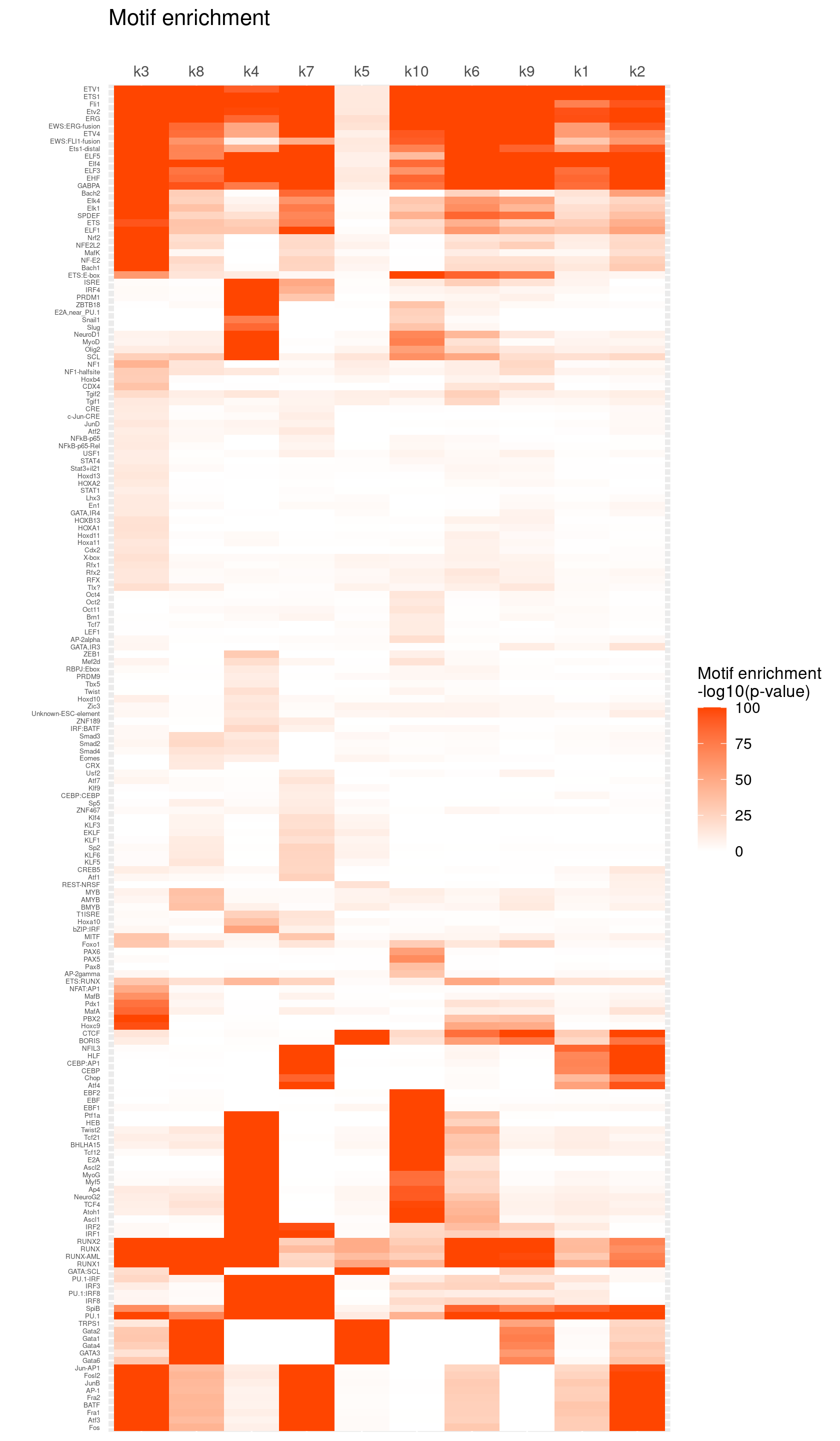
| Version | Author | Date |
|---|---|---|
| 3551232 | kevinlkx | 2022-03-09 |
# 181 out of 439 motifs included the heatmapTop enriched motifs
plots <- vector("list", ncol(motif_res$mlog10P))
names(plots) <- colnames(motif_res$mlog10P)

for( i in 1:length(plots)){
  plots[[i]] <- create_motif_enrichment_ranking_plot(motif_res, k = i,
                                                     max.overlaps = 20, subsample = FALSE)
}

do.call(plot_grid,plots)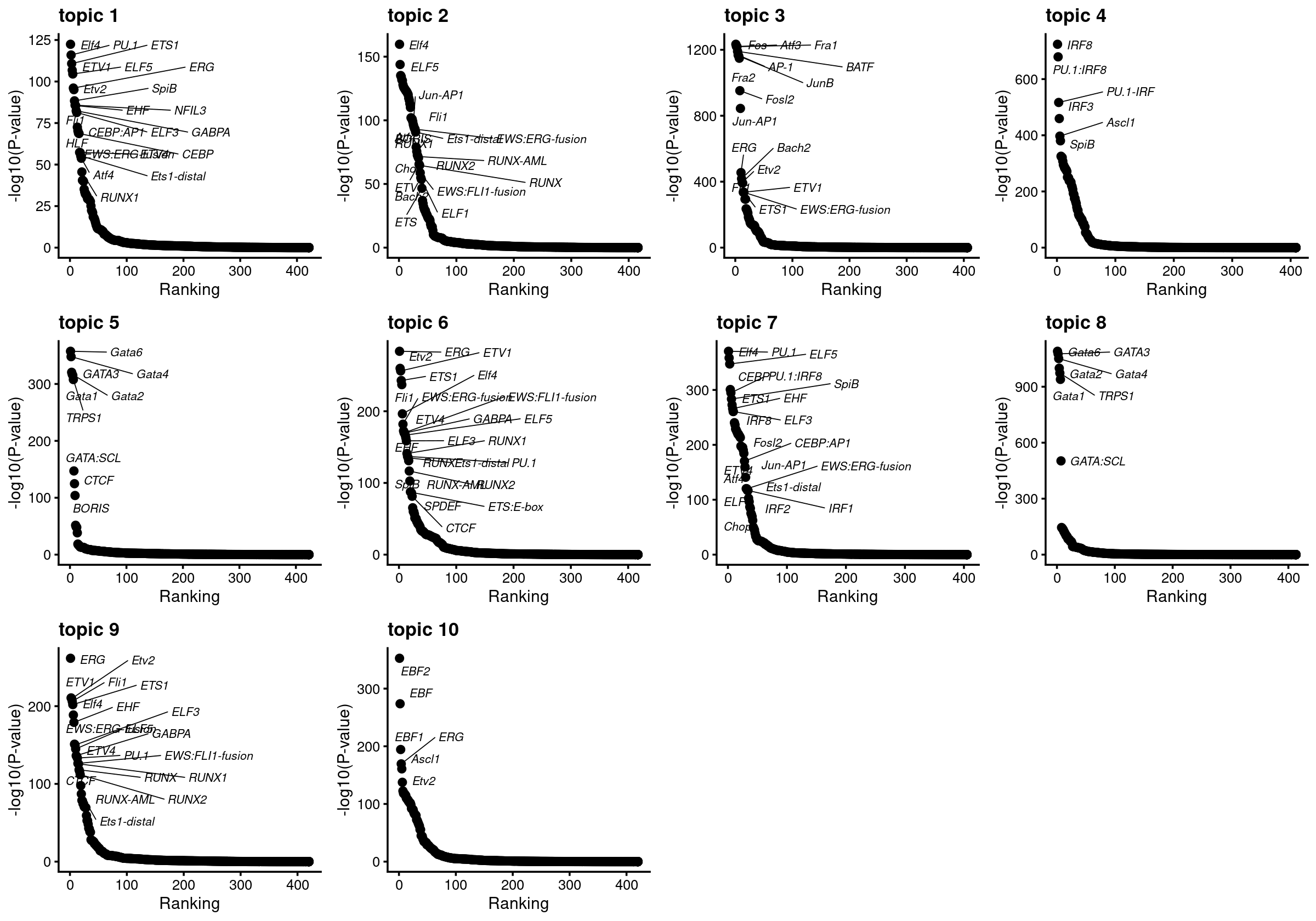
Motif enrichment result using top 2000 regions with largest logFC
Load and compile HOMER results across topics
postfit.dir <- "/project2/mstephens/kevinluo/scATACseq-topics/output/Buenrostro_2018/binarized/postfit_v2"
homer.dir <- paste0(postfit.dir, "/motifanalysis-Buenrostro2018-k=10/HOMER/DA_top2000_regions")
cat(sprintf("Directory of motif analysis result: %s \n", homer.dir))
homer_res_topics <- readRDS(file.path(homer.dir, "/homer_knownResults.rds"))
selected_regions <- readRDS(file.path(homer.dir, "/selected_regions.rds"))

# Compile Homer results (pvalue and ranking) across topics
motif_res <- compile_homer_motif_res(homer_res_topics)
saveRDS(motif_res, paste0(homer.dir, "/homer_motif_enrichment_results.rds"))
cat("compiled homer motif results are saved in", paste0(homer.dir, "/homer_motif_enrichment_results.rds \n"))
# Directory of motif analysis result: /project2/mstephens/kevinluo/scATACseq-topics/output/Buenrostro_2018/binarized/postfit_v2/motifanalysis-Buenrostro2018-k=10/HOMER/DA_top2000_regions
# compiled homer motif results are saved in /project2/mstephens/kevinluo/scATACseq-topics/output/Buenrostro_2018/binarized/postfit_v2/motifanalysis-Buenrostro2018-k=10/HOMER/DA_top2000_regions/homer_motif_enrichment_results.rdsTop 10 motifs for each topic
cat("Number of regions selected for each topic: \n")
print(mapply(nrow, selected_regions[1:(length(selected_regions)-1)]))

colnames_homer <- c("motif_name", "consensus", "P", "log10P", "Padj",  "num_target", "percent_target", "num_bg", "percent_bg")

top_motifs <- data.frame(matrix(nrow=10, ncol = length(homer_res_topics)))
colnames(top_motifs) <- names(homer_res_topics)
for (k in 1:length(homer_res_topics)){
  homer_res <- homer_res_topics[[k]]
  colnames(homer_res) <- colnames_homer
  homer_res <- homer_res %>% separate(motif_name, c("motif", "origin", "database"), "/")
  top_motifs[,k] <- head(homer_res$motif, 10)
}

DT::datatable(data.frame(rank = 1:10, top_motifs), rownames = F, caption = "Top 10 motifs enriched in each topic.")
# Number of regions selected for each topic:
# k1 k2 k3 k4 k5 k6 k7 k8 k9 k10
# 2000 2000 2000 2000 2000 2000 2000 2000 2000 2000Heatmap of motif enrichment -log10(p-value).
create_motif_enrichment_heatmap(motif_res, enrichment = "-log10(p-value)",
                                cluster_motifs = TRUE, cluster_topics = TRUE, motif_filter = 10, horizontal = FALSE,
                                enrichment_range = c(0,100), method_cluster = "average", font.size.motifs = 4, font.size.topics = 9)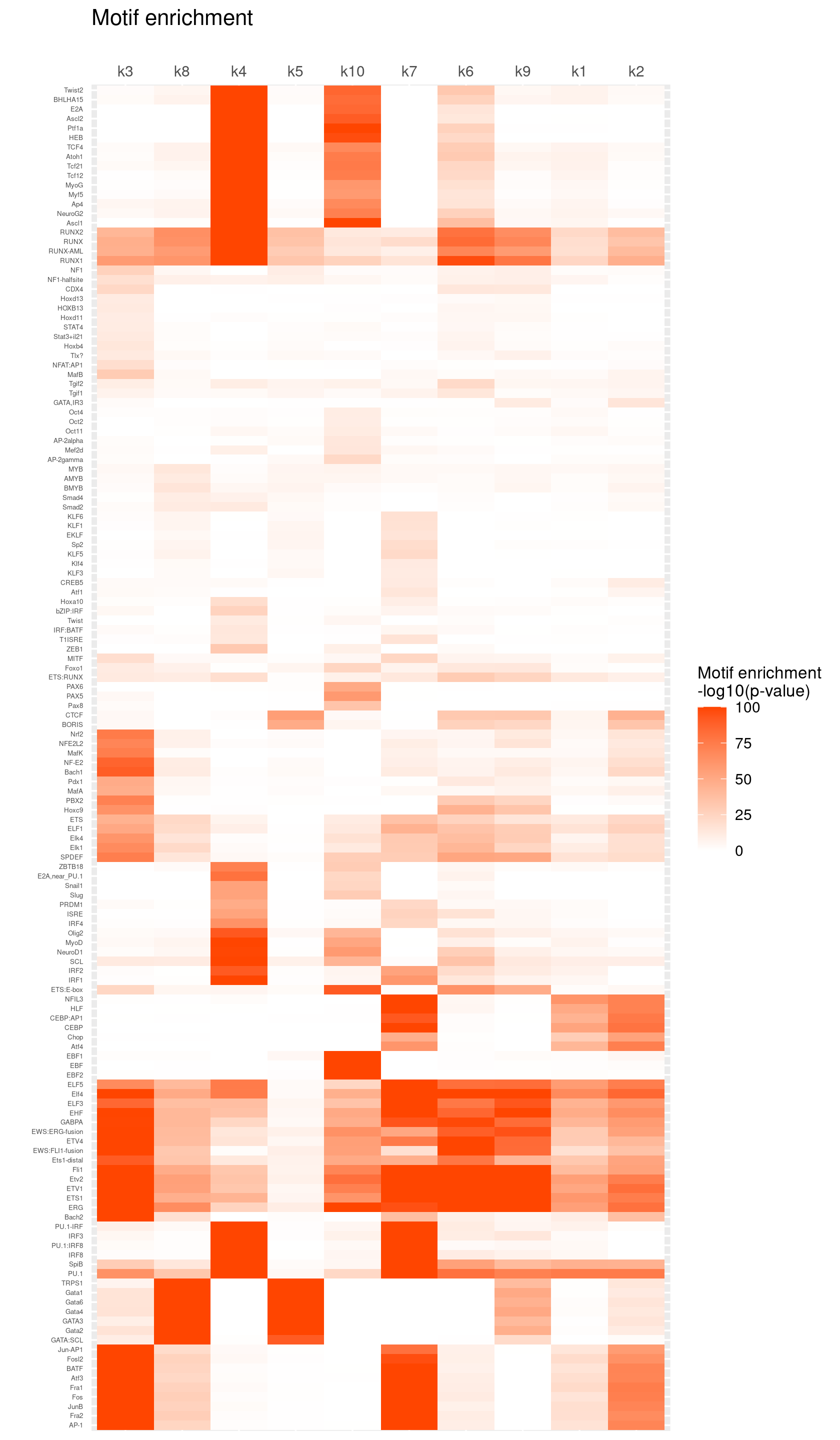
| Version | Author | Date |
|---|---|---|
| 3551232 | kevinlkx | 2022-03-09 |
# 142 out of 439 motifs included the heatmapTop enriched motifs
plots <- vector("list", ncol(motif_res$mlog10P))
names(plots) <- colnames(motif_res$mlog10P)

for( i in 1:length(plots)){
  plots[[i]] <- create_motif_enrichment_ranking_plot(motif_res, k = i,
                                                     max.overlaps = 20, subsample = FALSE)
}

do.call(plot_grid,plots)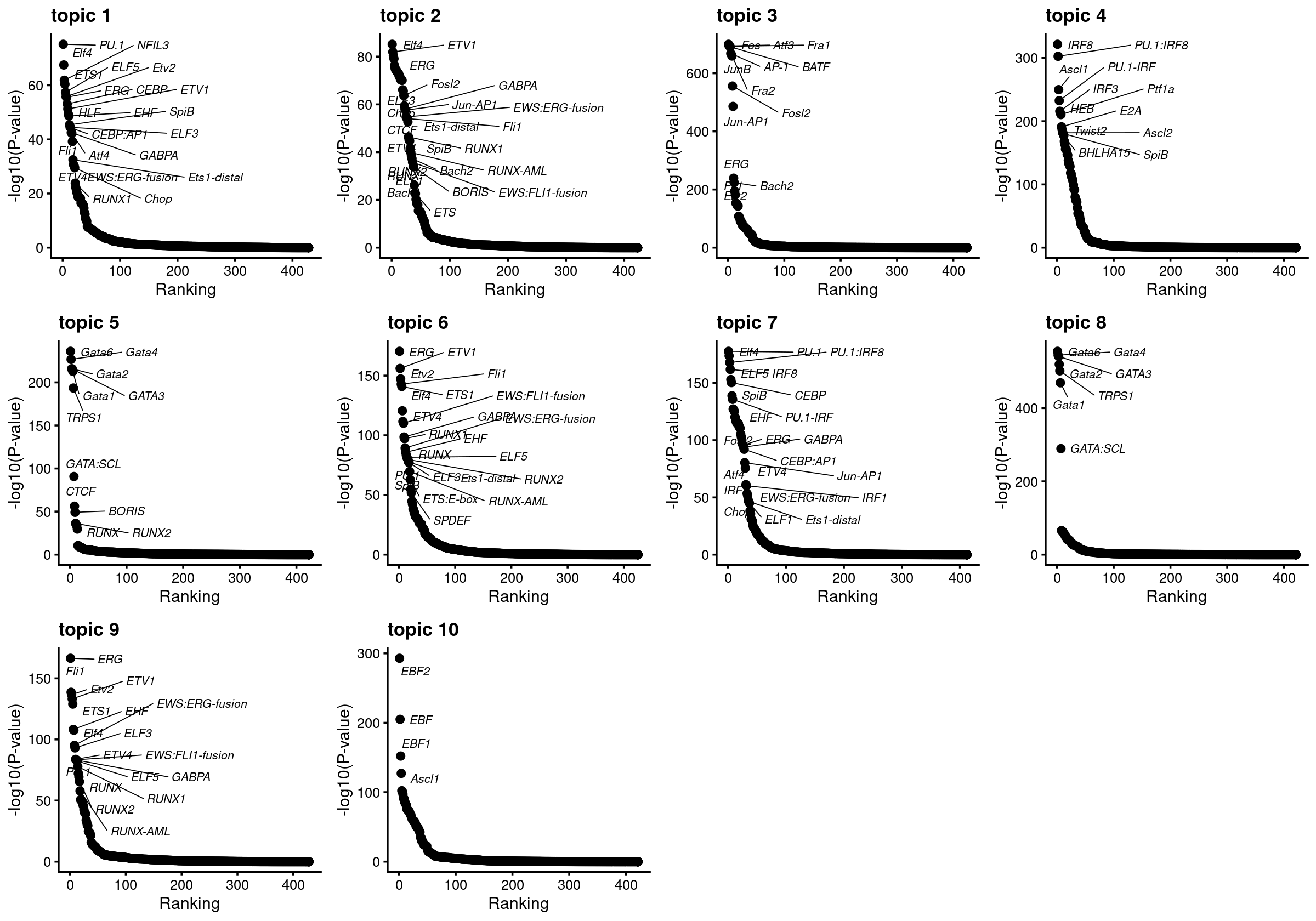
sessionInfo()# R version 4.0.4 (2021-02-15)
# Platform: x86_64-pc-linux-gnu (64-bit)
# Running under: Scientific Linux 7.4 (Nitrogen)
#
# Matrix products: default
# BLAS/LAPACK: /software/openblas-0.3.13-el7-x86_64/lib/libopenblas_haswellp-r0.3.13.so
#
# locale:
# [1] LC_CTYPE=en_US.UTF-8 LC_NUMERIC=C
# [3] LC_TIME=en_US.UTF-8 LC_COLLATE=en_US.UTF-8
# [5] LC_MONETARY=en_US.UTF-8 LC_MESSAGES=en_US.UTF-8
# [7] LC_PAPER=en_US.UTF-8 LC_NAME=C
# [9] LC_ADDRESS=C LC_TELEPHONE=C
# [11] LC_MEASUREMENT=en_US.UTF-8 LC_IDENTIFICATION=C
#
# attached base packages:
# [1] stats graphics grDevices utils datasets methods base
#
# other attached packages:
# [1] reshape2_1.4.4 DT_0.20 plotly_4.10.0 cowplot_1.1.1
# [5] ggrepel_0.9.1 ggplot2_3.3.5 tidyr_1.1.4 dplyr_1.0.8
# [9] fastTopics_0.6-97 Matrix_1.4-0 workflowr_1.7.0
#
# loaded via a namespace (and not attached):
# [1] Rtsne_0.15 colorspace_2.0-3 ellipsis_0.3.2
# [4] class_7.3-20 rprojroot_2.0.2 fs_1.5.2
# [7] rstudioapi_0.13 farver_2.1.0 listenv_0.8.0
# [10] MatrixModels_0.5-0 prodlim_2019.11.13 fansi_1.0.2
# [13] lubridate_1.8.0 codetools_0.2-18 splines_4.0.4
# [16] knitr_1.37 jsonlite_1.7.3 pROC_1.18.0
# [19] mcmc_0.9-7 caret_6.0-90 ashr_2.2-47
# [22] uwot_0.1.11 compiler_4.0.4 httr_1.4.2
# [25] assertthat_0.2.1 fastmap_1.1.0 lazyeval_0.2.2
# [28] cli_3.2.0 later_1.3.0 prettyunits_1.1.1
# [31] htmltools_0.5.2 quantreg_5.86 tools_4.0.4
# [34] coda_0.19-4 gtable_0.3.0 glue_1.6.2
# [37] Rcpp_1.0.8 jquerylib_0.1.4 vctrs_0.3.8
# [40] nlme_3.1-155 conquer_1.2.1 crosstalk_1.2.0
# [43] iterators_1.0.13 timeDate_3043.102 gower_0.2.2
# [46] xfun_0.29 stringr_1.4.0 globals_0.14.0
# [49] ps_1.6.0 lifecycle_1.0.1 irlba_2.3.5
# [52] future_1.23.0 getPass_0.2-2 MASS_7.3-55
# [55] scales_1.1.1 ipred_0.9-12 hms_1.1.1
# [58] promises_1.2.0.1 parallel_4.0.4 SparseM_1.81
# [61] yaml_2.2.2 pbapply_1.5-0 sass_0.4.0
# [64] rpart_4.1-15 stringi_1.7.6 SQUAREM_2021.1
# [67] highr_0.9 foreach_1.5.1 lava_1.6.10
# [70] truncnorm_1.0-8 rlang_1.0.1 pkgconfig_2.0.3
# [73] matrixStats_0.61.0 evaluate_0.14 lattice_0.20-45
# [76] invgamma_1.1 purrr_0.3.4 labeling_0.4.2
# [79] recipes_0.1.17 htmlwidgets_1.5.4 processx_3.5.2
# [82] tidyselect_1.1.2 parallelly_1.30.0 plyr_1.8.6
# [85] magrittr_2.0.2 R6_2.5.1 generics_0.1.2
# [88] DBI_1.1.2 pillar_1.7.0 whisker_0.4
# [91] withr_2.4.3 survival_3.2-13 mixsqp_0.3-43
# [94] nnet_7.3-17 tibble_3.1.6 future.apply_1.8.1
# [97] crayon_1.5.0 utf8_1.2.2 rmarkdown_2.11
# [100] progress_1.2.2 grid_4.0.4 data.table_1.14.2
# [103] callr_3.7.0 git2r_0.29.0 ModelMetrics_1.2.2.2
# [106] digest_0.6.29 httpuv_1.6.5 MCMCpack_1.6-0
# [109] RcppParallel_5.1.5 stats4_4.0.4 munsell_0.5.0
# [112] viridisLite_0.4.0 bslib_0.3.1 quadprog_1.5-8