Initial exploration of the human brain dataset: committed OPC cells

Last updated: 2024-11-17

Checks: 7 0

Knit directory: single-cell-jamboree/analysis/

This reproducible R Markdown analysis was created with workflowr (version 1.7.1). The Checks tab describes the reproducibility checks that were applied when the results were created. The Past versions tab lists the development history.

R Markdown file: up-to-date

Great! Since the R Markdown file has been committed to the Git repository, you know the exact version of the code that produced these results.

Environment: empty

Great job! The global environment was empty. Objects defined in the global environment can affect the analysis in your R Markdown file in unknown ways. For reproduciblity it’s best to always run the code in an empty environment.

Seed: set.seed(1)

The command set.seed(1) was run prior to running the code in the R Markdown file. Setting a seed ensures that any results that rely on randomness, e.g. subsampling or permutations, are reproducible.

Session information: recorded

Great job! Recording the operating system, R version, and package versions is critical for reproducibility.

Cache: none

Nice! There were no cached chunks for this analysis, so you can be confident that you successfully produced the results during this run.

File paths: relative

Great job! Using relative paths to the files within your workflowr project makes it easier to run your code on other machines.

Repository version: 8280492

Great! You are using Git for version control. Tracking code development and connecting the code version to the results is critical for reproducibility.

The results in this page were generated with repository version 8280492. See the Past versions tab to see a history of the changes made to the R Markdown and HTML files.

Note that you need to be careful to ensure that all relevant files for the analysis have been committed to Git prior to generating the results (you can use wflow_publish or wflow_git_commit). workflowr only checks the R Markdown file, but you know if there are other scripts or data files that it depends on. Below is the status of the Git repository when the results were generated:


Ignored files:
    Ignored:    .Rhistory
    Ignored:    .Rproj.user/
    Ignored:    analysis/.Rhistory
    Ignored:    data/.Rhistory

Untracked files:
    Untracked:  .DS_Store
    Untracked:  .gitignore
    Untracked:  analysis/.DS_Store
    Untracked:  analysis/human_brain_COP_cells_fit.RData
    Untracked:  code/read_gene_set_data.R
    Untracked:  data/.DS_Store
    Untracked:  data/Homo_sapiens.gene_info.gz
    Untracked:  data/human_brain_COP_cells_fit.RData

Note that any generated files, e.g. HTML, png, CSS, etc., are not included in this status report because it is ok for generated content to have uncommitted changes.

These are the previous versions of the repository in which changes were made to the R Markdown (analysis/human_brain_COP_cells.Rmd) and HTML (docs/human_brain_COP_cells.html) files. If you’ve configured a remote Git repository (see ?wflow_git_remote), click on the hyperlinks in the table below to view the files as they were in that past version.

File	Version	Author	Date	Message
Rmd	8280492	junmingguan	2024-11-17	workflowr::wflow_publish("analysis/human_brain_COP_cells.Rmd")
html	7a353a3	junmingguan	2024-11-09	Build site.
Rmd	e8fc53f	junmingguan	2024-11-09	workflowr::wflow_publish("human_brain_COP_cells.Rmd")

Introduction

This single-nucleus RNA seq dataset is from the paper “Transcriptomic diversity of cell types across the adult human brain” (Siletti, 2023). around 3 millions nuclei were collected from around 100 dissections from the following areas of brains of 3 donors:

Forebrain:
- cerebral cortex
- cerebral nuclei
- hypothalamus
- hippocampus formation
- thalamus complex
Midbrain
Hindbrain:
- pons
- cerebellum
- Myelencephalon (Medulla)
Spinal cord

The authors performed hierarchical graph-based clustering, grouping the cells into superclusters, clusters, and subclusters. The data can be accessed here, with files organized by supercluster or by dissection.

This exploratory analysis focuses on committed oligodendrocyte precursor (COP) cells (see https://cellxgene.cziscience.com/e/f16f4108-7873-4035-9989-3748da1a7ff1.cxg/). There are 4,720 cells and 2,1462 genes (after QC) in the dataset.

library(Matrix)
# library(MatrixExtra)
library(flashier)
library(fastTopics)
library(ggplot2)
library(cowplot)
library(dplyr)
library(readr)
library(knitr)
# Warning: package 'knitr' was built under R version 4.3.3

Load data and fit

# Taken from https://github.com/stephenslab/pathways/blob/master/inst/code/read_gene_set_data.R
read_gene_info <- function (file) {
  
  # Read the data into a data frame.
  out <- suppressMessages(read_delim(file,delim = "\t",col_names = TRUE))
  class(out) <- "data.frame"
  dbXrefs    <- out$dbXrefs
  out        <- out[c("GeneID","Symbol","Synonyms","chromosome")]
  
  # Set any entries with a single hyphen to NA, and convert the
  # "chromosome" column to a factor.
  out$chromosome[out$chromosome == "-"] <- NA
  out$Synonyms[out$Synonyms == "-"]     <- NA
  dbXrefs[dbXrefs == "-"]               <- NA
  out <- transform(out,chromosome = factor(chromosome))
  
  # Extract the Ensembl ids. Note that a small number of genes map to
  # more than one Ensembl id; in those cases, we retain the first
  # Ensembl id only.
  dbXrefs <- strsplit(dbXrefs,"|",fixed = TRUE)
  out$Ensembl <- sapply(dbXrefs,function (x) {
    i <- which(substr(x,1,8) == "Ensembl:")
    if (length(i) > 0)
      return(substr(x[i[1]],9,nchar(x[i[1]])))
    else
      return(as.character(NA))
  })
  
  # For human genes, extract the HGNC (HUGO Gene Nomenclature
  # Committee) ids.
  out$HGNC <- sapply(dbXrefs,function (x) {
    i <- which(substr(x,1,10) == "HGNC:HGNC:")
    if (length(i) > 0)
      return(substr(x[i[1]],6,nchar(x[i[1]])))
    else
      return(as.character(NA))
  })
  
  # Return the processed gene data.
  return(out)
}

homo_sapien_geno_info <- read_gene_info('../data/Homo_sapiens.gene_info.gz')
data <- readRDS('../data/human_brain_COP_cells.rds')
counts <- t(data$RNA$data)
# Warning: package 'SeuratObject' was built under R version 4.3.3

# Keep only protein-coding genes and remove those without nonzero counts
reduced_counts <- 
  counts[, colnames(counts) %in% homo_sapien_geno_info$Ensembl]
cols_to_keep <- colSums(reduced_counts != 0, na.rm = TRUE) > 0
reduced_counts <- reduced_counts[, cols_to_keep]
load('../data/human_brain_COP_cells_fit.RData')

map_tissue <- function(tissue) {
  if (tissue %in% c("cerebral cortex", "cerebral nuclei", "hypothalamus", 
                    "hippocampal formation", "thalamic complex")) {
    return("forebrain")
  } else if (tissue == "midbrain") {
    return("midbrain")
  } else if (tissue %in% c("pons", "cerebellum", "myelencephalon")) {
    return("hindbrain")
  } else if (tissue == "spinal cord") {
    return("spinal cord")
  } else {
    return(NA)
  }
}

regions <- sapply(data$tissue, map_tissue)

t-SNE and UMAP

The dataset includes precomputed tSNE and UMAP embeddings, allowing us to plot them directly. We can color the cells by tissue, by region, or by cluster.

t-SNE

# colors <- brewer.pal(length(unique(data$tissue)), "Paired")
colors <-  c('#756bb1', '#1c9099', '#d95f0e', '#edf8b1', '#dd1c77', '#636363', '#a1d99b', '#fa9fb5', '#fec44f', '#de2d26')
ggplot(Embeddings(data$tSNE) , aes(x = TSNE_1, y = TSNE_2, color = data$tissue)) +
  geom_point(alpha = 0.7) +
  labs(title = "t-SNE Plot Colored by Tissue Type", x = "t-SNE 1", y = "t-SNE 2") +
  theme_minimal() +
  scale_color_manual(values = colors)

Version	Author	Date
7a353a3	junmingguan	2024-11-09


# colors <- brewer.pal(length(unique(regions)), "Set1")
# ggplot(Embeddings(data$tSNE) , aes(x = TSNE_1, y = TSNE_2, color = regions)) +
#   geom_point(alpha = 0.7) +
#   labs(title = "t-SNE Plot Colored by Tissue Type", x = "t-SNE 1", y = "t-SNE 2") +
#   theme_minimal() +
#   scale_color_manual(values = colors)

# colors <- brewer.pal(length(unique(data$cluster_id)), "Paired")
colors <-  c('#756bb1', '#1c9099', '#d95f0e', '#edf8b1', '#dd1c77', '#636363', '#a1d99b')
ggplot(Embeddings(data$tSNE) , aes(x = TSNE_1, y = TSNE_2, color = data$cluster_id)) +
  geom_point(alpha = 0.7) +
  labs(title = "t-SNE Plot Colored by Cluster", x = "t-SNE 1", y = "t-SNE 2") +
  theme_minimal() +
  scale_color_manual(values = colors)

Version	Author	Date
7a353a3	junmingguan	2024-11-09

UMAP

# colors <- brewer.pal(length(unique(data$tissue)), "Paired")
colors <-  c('#756bb1', '#1c9099', '#d95f0e', '#edf8b1', '#dd1c77', '#636363', '#a1d99b', '#fa9fb5', '#fec44f', '#de2d26')
ggplot(Embeddings(data$UMAP) , aes(x = UMAP_1, y = UMAP_2, color = data$tissue)) +
  geom_point(alpha = 0.7) +
  labs(title = "UMAP Plot Colored by Tissue Type", x = "UMAP 1", y = "UMAP 2") +
  theme_minimal() +
  scale_color_manual(values = colors)

Version	Author	Date
7a353a3	junmingguan	2024-11-09


# ggplot(Embeddings(data$UMAP) , aes(x = UMAP_1, y = UMAP_2, color = regions)) +
#   geom_point(alpha = 0.7) +
#   labs(title = "UMAP Plot Colored by Tissue Type", x = "UMAP 1", y = "UMAP 2") +
#   theme_minimal() +
#   scale_color_manual(values = rainbow(length(unique(regions))))

# colors <- brewer.pal(length(unique(data$cluster_id)), "Paired")
colors <-  c('#756bb1', '#1c9099', '#d95f0e', '#edf8b1', '#dd1c77', '#636363', '#a1d99b')
ggplot(Embeddings(data$UMAP) , aes(x = UMAP_1, y = UMAP_2, color = data$cluster_id)) +
  geom_point(alpha = 0.7) +
  labs(title = "UMAP Plot Colored by Cluster", x = "UMAP 1", y = "UMAP 2") +
  theme_minimal() +
  scale_color_manual(values = colors)

Version	Author	Date
7a353a3	junmingguan	2024-11-09

Flashier

NMF

Redefine subcluster ids so that the hierarchical structure is clearer

# M <- table(data$subcluster_id, data$cluster_id)
# M
subcluster_id <- as.vector(data$subcluster_id)
subcluster_id[subcluster_id == '3033'] <- '37.1'
subcluster_id[subcluster_id == '3035'] <- '37.2'
subcluster_id[subcluster_id == '3036'] <- '37.3'
subcluster_id[subcluster_id == '3037'] <- '37.4'
subcluster_id[subcluster_id == '3038'] <- '37.5'

subcluster_id[subcluster_id == '3030'] <- '38.1'
subcluster_id[subcluster_id == '3031'] <- '38.2'
subcluster_id[subcluster_id == '3032'] <- '38.3'
subcluster_id[subcluster_id == '3034'] <- '38.4'

subcluster_id[subcluster_id == '3027'] <- '39.1'
subcluster_id[subcluster_id == '3028'] <- '39.2'
subcluster_id[subcluster_id == '3029'] <- '39.3'

subcluster_id[subcluster_id == '3014'] <- '41.1'
subcluster_id[subcluster_id == '3015'] <- '42.2'

subcluster_id[subcluster_id == '3007'] <- '42.1'
subcluster_id[subcluster_id == '3008'] <- '42.2'
subcluster_id[subcluster_id == '3009'] <- '42.3'
subcluster_id[subcluster_id == '3010'] <- '42.4'

subcluster_id[subcluster_id == '3006'] <- '43.1'

subcluster_id[subcluster_id == '3195'] <- '75.1'
subcluster_id[subcluster_id == '3196'] <- '75.2'
subcluster_id <- factor(subcluster_id)

flash_plot_scree(flashier_fit)

Version	Author	Date
7a353a3	junmingguan	2024-11-09



plot(flashier_fit, 
     plot_type = "heatmap",
     pm_which = "loadings", 
     pm_groups = data$cluster_id,
     gap = 25)

Version	Author	Date
7a353a3	junmingguan	2024-11-09


plot(flashier_fit, 
     plot_type = "histogram",
     pm_which = "loadings", 
     pm_groups = data$cluster_id,
     bins = 25)

Version	Author	Date
7a353a3	junmingguan	2024-11-09

plot(flashier_fit, 
     plot_type = "structure",
     pm_which = "loadings", 
     pm_groups = data$cluster_id,
     bins = 30, gap = 70)

Version	Author	Date
7a353a3	junmingguan	2024-11-09


plot(flashier_fit, 
     plot_type = "structure",
     pm_which = "loadings", 
     pm_groups = subcluster_id,
     bins = 60, gap = 100)

Version	Author	Date
7a353a3	junmingguan	2024-11-09

vals <- ldf(flashier_fit,type="m")
ncells <- colSums(vals$L>0.1)
ncells
#  [1] 4720 3101 1557   79 2060 1641 1281    1    5    1    4    2 1795

Several factors are load on only a small number of cells.

Removing those factors from the structure plots:

plot(flashier_fit, 
     kset = which(ncells > 5),
     plot_type = "structure",
     pm_which = "loadings", 
     pm_groups = data$cluster_id,
     bins = 30, gap = 70)

Version	Author	Date
7a353a3	junmingguan	2024-11-09


plot(flashier_fit, 
     kset = which(ncells > 5),
     plot_type = "structure",
     pm_which = "loadings", 
     pm_groups = subcluster_id,
     bins = 60, gap = 100)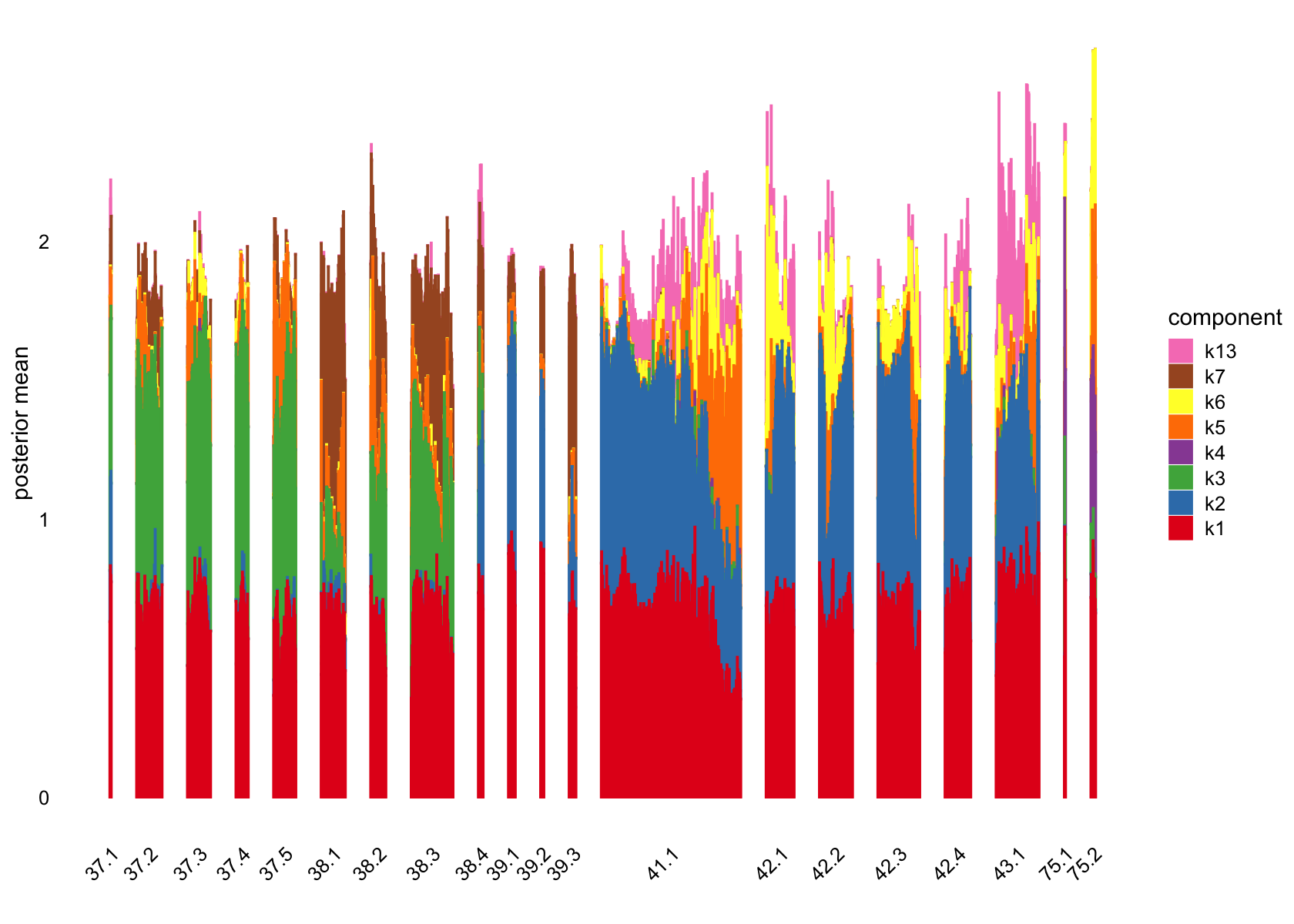

Version	Author	Date
7a353a3	junmingguan	2024-11-09

Showing those factors in the structure plots:

plot(flashier_fit, 
     kset = which(ncells <= 5),
     plot_type = "structure",
     pm_which = "loadings", 
     pm_groups = data$cluster_id,
     bins = 30, gap = 70)

Version	Author	Date
7a353a3	junmingguan	2024-11-09


plot(flashier_fit, 
     kset = which(ncells <= 5),
     plot_type = "structure",
     pm_which = "loadings", 
     pm_groups = subcluster_id,
     bins = 60, gap = 100)

Version	Author	Date
7a353a3	junmingguan	2024-11-09

Top 10 driving genes for factors that are loading on a small number of cells

low_factors <- which(ncells <= 5)
top10_genes <- list()
for (f in low_factors) {
  factor_name <- paste('Factor', f)
  genes <- head(sort(vals$F[, f], decreasing = T), 10)
  top10_ensembl <- names(genes)
  top10_symbol <- homo_sapien_geno_info$Symbol[match(top10_ensembl, homo_sapien_geno_info$Ensembl)]
  top10_genes[[factor_name]] <- top10_symbol
  
  factor_name <- paste('Factor', f, 'score')
  top10_genes[[factor_name]] <- as.vector(genes)
  
}
top10_genes %>% as.data.frame() %>% kable()

loadings on UMAP by factor

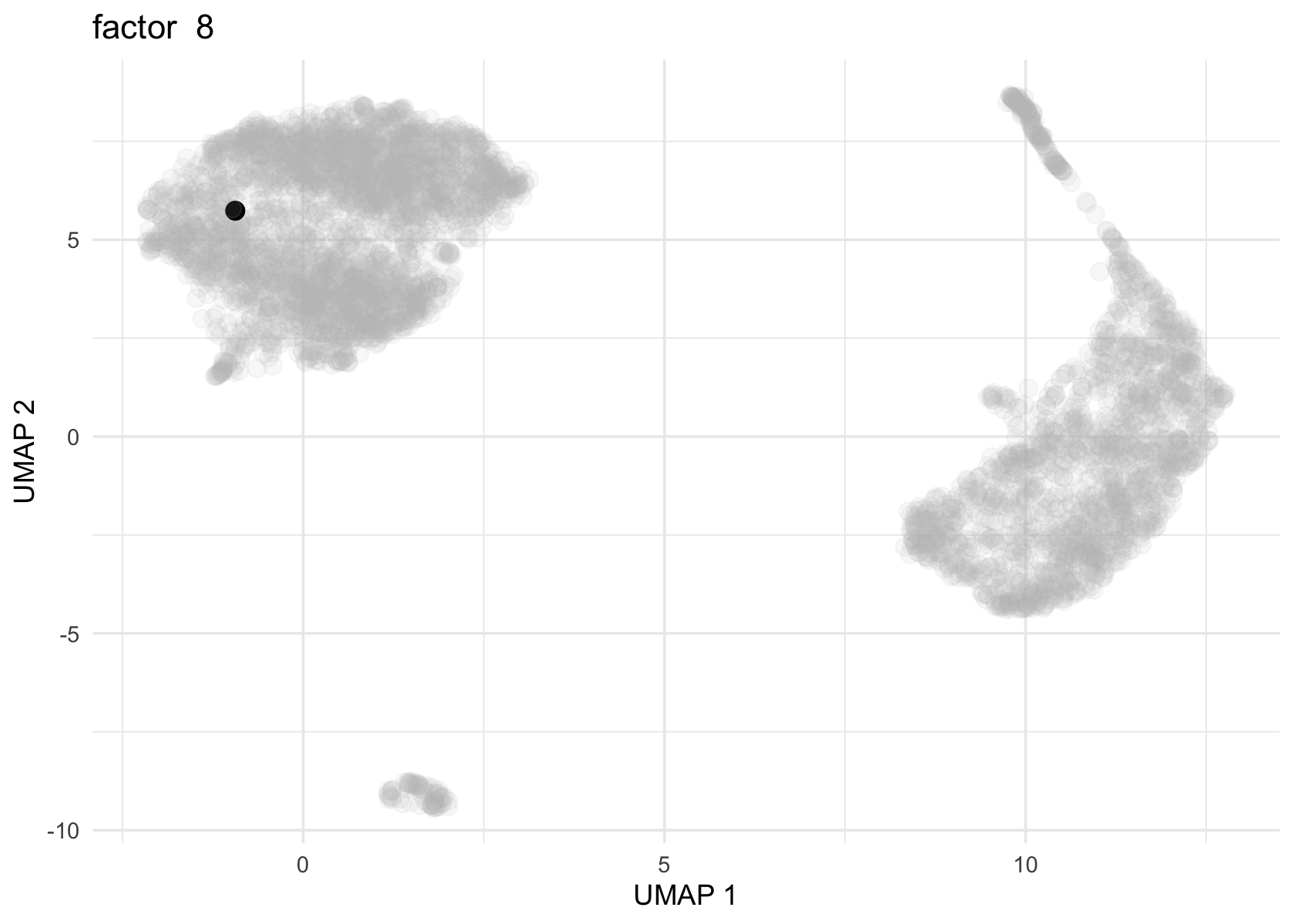
Factor 2, 3 and 4 are heavily loaded, whereas factor 8 and 9 are loaded on a single cell.

umap <- Embeddings(data$UMAP)
source('../code/plot_loadings_on_umap.R')

for (f in c(2, 3, 4, 8, 9)) {
  loading <- vals$L[, f]
  p <- plot_loadings_on_umap(umap, loading, f)
  print(p)
}

Semi-NMF

flash_plot_scree(flashier_fit_semi)

Version	Author	Date
7a353a3	junmingguan	2024-11-09



plot(flashier_fit_semi, 
     plot_type = "heatmap",
     pm_which = "loadings", 
     pm_groups = data$cluster_id,
     gap = 25)

Version	Author	Date
7a353a3	junmingguan	2024-11-09


plot(flashier_fit_semi, 
     plot_type = "histogram",
     pm_which = "loadings", 
     pm_groups = data$cluster_id,
     bins = 25)

Version	Author	Date
7a353a3	junmingguan	2024-11-09

plot(flashier_fit_semi, 
     plot_type = "structure",
     pm_which = "loadings", 
     pm_groups = data$cluster_id,
     bins = 30, gap = 70)

Version	Author	Date
7a353a3	junmingguan	2024-11-09


plot(flashier_fit_semi, 
     plot_type = "structure",
     pm_which = "loadings", 
     pm_groups = subcluster_id,
     bins = 60, gap = 100)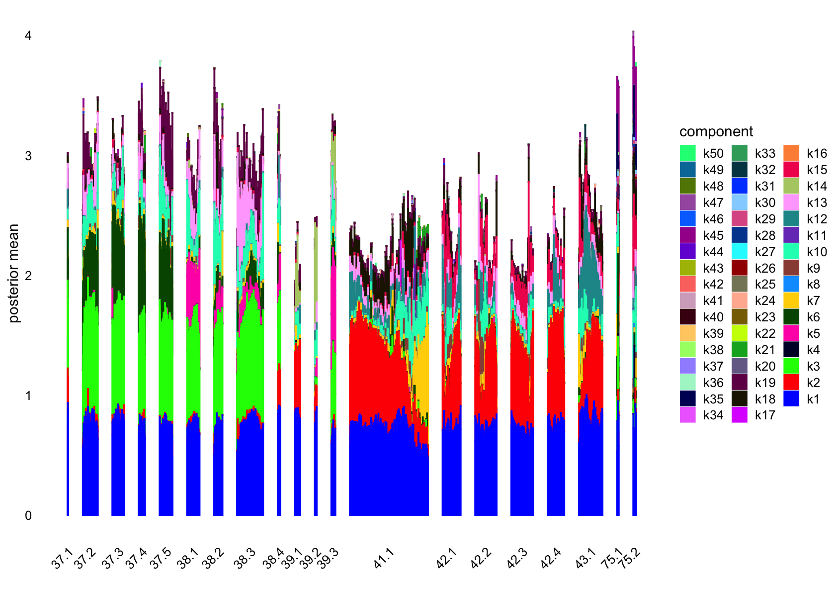

Version	Author	Date
7a353a3	junmingguan	2024-11-09

vals_semi <- ldf(flashier_fit_semi, type="m")
ncells_semi <- colSums(vals_semi$L>0.1)
ncells_semi
#  [1] 4720 3121 1700    3  559 1208  769    1  324 2350    1 1469 1799  177 1591
# [16]    1    1 1838 1886    3   68    1    2    1    3    1    2    5    2    1
# [31]    1    2    1    1   54    1    5    1    1    1    2    2    1    1   59
# [46]    2    2    3    1    3

Several factors are load on only a small number of cells.

Removing those factors from the structure plots:

plot(flashier_fit_semi, 
     kset = which(ncells_semi > 5),
     plot_type = "structure",
     pm_which = "loadings", 
     pm_groups = data$cluster_id,
     bins = 30, gap = 70)

Version	Author	Date
7a353a3	junmingguan	2024-11-09


plot(flashier_fit_semi, 
     kset = which(ncells_semi > 5),
     plot_type = "structure",
     pm_which = "loadings", 
     pm_groups = subcluster_id,
     bins = 60, gap = 100)

Version	Author	Date
7a353a3	junmingguan	2024-11-09

Showing factors that are only loaded on a small number of cells:

plot(flashier_fit_semi, 
     kset = which(ncells_semi <= 5),
     plot_type = "structure",
     pm_which = "loadings", 
     pm_groups = data$cluster_id,
     bins = 30, gap = 70)

Version	Author	Date
7a353a3	junmingguan	2024-11-09


plot(flashier_fit_semi, 
     kset = which(ncells_semi <= 5),
     plot_type = "structure",
     pm_which = "loadings", 
     pm_groups = subcluster_id,
     bins = 60, gap = 100)

Version	Author	Date
7a353a3	junmingguan	2024-11-09

Top 10 driving genes for factors that are loading on a small number of cells

low_factors <- which(ncells_semi <= 5)
top10_genes <- list()
for (f in low_factors) {
  factor_name <- paste('Factor', f)
  genes <- head(sort(vals_semi$F[, f], decreasing = T), 10)
  top10_ensembl <- names(genes)
  top10_symbol <- homo_sapien_geno_info$Symbol[match(top10_ensembl, homo_sapien_geno_info$Ensembl)]
  top10_genes[[factor_name]] <- top10_symbol
  
  factor_name <- paste('Factor', f, 'score')
  top10_genes[[factor_name]] <- as.vector(genes)
  
}
top10_genes %>% as.data.frame() %>% kable()

loadings on UMAP by factor

Factor 2 and 3 are heavily loaded, whereas factor 4 and 4 are loaded on a few cells.

umap <- Embeddings(data$UMAP)
source('../code/plot_loadings_on_umap.R')

for (f in c(2, 3, 4, 8)) {
  loading <- vals_semi$L[, f]
  p <- plot_loadings_on_umap(umap, loading, f)
  print(p)
}

Comparison


plot(flashier_fit, 
     kset = which(ncells > 5),
     plot_type = "structure",
     pm_which = "loadings", 
     pm_groups = data$cluster_id,
     bins = 30, gap = 70)

Version	Author	Date
7a353a3	junmingguan	2024-11-09


plot(flashier_fit_semi, 
     kset = which(ncells_semi > 5),
     plot_type = "structure",
     pm_which = "loadings", 
     pm_groups = data$cluster_id,
     bins = 30, gap = 70)

Version	Author	Date
7a353a3	junmingguan	2024-11-09


# plot_grid(p1, p2, ncol = 1, align = "v", axis = "lr", rel_heights = c(1, 1))

FastTopics

plot_progress(fasttopics_fit,x = "iter",add.point.every = 10,colors = "black") +
  theme_cowplot(font_size = 10)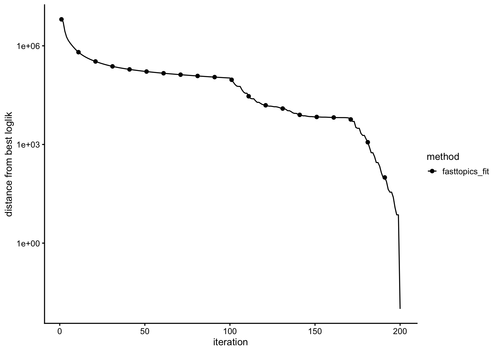

Version	Author	Date
7a353a3	junmingguan	2024-11-09

loglik <- loglik_multinom_topic_model(reduced_counts, fasttopics_fit)
pdat <- data.frame(loglik)
ggplot(pdat,aes(loglik)) +
  geom_histogram(bins = 64,color = "white",fill = "black",size = 0.25) +
  labs(y = "number of cells") +
  theme_cowplot(font_size = 10)
# Warning: Using `size` aesthetic for lines was deprecated in ggplot2 3.4.0.
# ℹ Please use `linewidth` instead.
# This warning is displayed once every 8 hours.
# Call `lifecycle::last_lifecycle_warnings()` to see where this warning was
# generated.

Version	Author	Date
7a353a3	junmingguan	2024-11-09


# subpop_colors <- c("dodgerblue","forestgreen","darkmagenta","skyblue","gold", )
subpop_colors <- c("red", "blue", "green", "purple", "orange", "pink", "cyan", "brown", "yellow", "darkgreen")

pdat <- data.frame(loglik = loglik,subpop = data$tissue)
ggplot(pdat,aes(x = loglik,fill = subpop)) +
  geom_histogram(bins = 64,color = "white",size = 0.25) +
  scale_fill_manual(values = subpop_colors) +
  labs(y = "number of cells") +
  theme_cowplot(font_size = 10)

Version	Author	Date
7a353a3	junmingguan	2024-11-09

structure_plot(fasttopics_fit, grouping = data$cluster_id, gap = 70)

Version	Author	Date
7a353a3	junmingguan	2024-11-09

structure_plot(fasttopics_fit, grouping = subcluster_id, gap = 70)

Version	Author	Date
7a353a3	junmingguan	2024-11-09

ncells_ft <- colSums(fasttopics_fit$L>0.1)
ncells_ft
#   k1   k2   k3   k4   k5   k6   k7   k8   k9  k10  k11  k12  k13  k14  k15  k16 
#  127   97  876  156 1019  115  405   12  171  112 1734  315  141   20  112   35 
#  k17  k18  k19  k20  k21  k22  k23  k24  k25  k26  k27  k28  k29  k30  k31  k32 
#   46   65  143  484  322  281 1008  127   66  347  107  128   38  612  517  202 
#  k33  k34  k35  k36  k37  k38  k39  k40  k41  k42  k43  k44  k45  k46  k47  k48 
#  196  148  877   24   70   28  204  370  259  189   58   44  120  402   72  433 
#  k49  k50 
#   22  313

No factors that are loaded on a single cells. Still there are a couple that are loaded on a small number of cells, e.g., k8.

GBCD

TODO

# source("../code/fit_cov_ebnmf.R")
# 
# fit.gbcd <-
#   flash_fit_cov_ebnmf(Y = reduced_counts, Kmax = 7,
#                       prior = flash_ebnm(prior_family = "generalized_binary",
#                                          scale = 0.04),
#                       extrapolate = FALSE)

sessionInfo()
# R version 4.3.1 (2023-06-16)
# Platform: aarch64-apple-darwin20 (64-bit)
# Running under: macOS Sonoma 14.5
# 
# Matrix products: default
# BLAS:   /Library/Frameworks/R.framework/Versions/4.3-arm64/Resources/lib/libRblas.0.dylib 
# LAPACK: /Library/Frameworks/R.framework/Versions/4.3-arm64/Resources/lib/libRlapack.dylib;  LAPACK version 3.11.0
# 
# locale:
# [1] en_US.UTF-8/en_US.UTF-8/en_US.UTF-8/C/en_US.UTF-8/en_US.UTF-8
# 
# time zone: America/Chicago
# tzcode source: internal
# 
# attached base packages:
# [1] stats     graphics  grDevices utils     datasets  methods   base     
# 
# other attached packages:
#  [1] SeuratObject_5.0.2 sp_2.1-4           knitr_1.48         readr_2.1.4       
#  [5] dplyr_1.1.4        cowplot_1.1.3      ggplot2_3.5.1      fastTopics_0.6-192
#  [9] flashier_1.0.54    ebnm_1.1-34        Matrix_1.6-4      
# 
# loaded via a namespace (and not attached):
#  [1] pbapply_1.7-2        rlang_1.1.4          magrittr_2.0.3      
#  [4] git2r_0.35.0         horseshoe_0.2.0      compiler_4.3.1      
#  [7] vctrs_0.6.5          quadprog_1.5-8       stringr_1.5.1       
# [10] pkgconfig_2.0.3      crayon_1.5.3         fastmap_1.2.0       
# [13] labeling_0.4.3       utf8_1.2.4           promises_1.3.0      
# [16] rmarkdown_2.28       tzdb_0.4.0           purrr_1.0.2         
# [19] bit_4.0.5            xfun_0.48            cachem_1.1.0        
# [22] trust_0.1-8          jsonlite_1.8.9       progress_1.2.3      
# [25] highr_0.11           later_1.3.2          irlba_2.3.5.1       
# [28] parallel_4.3.1       prettyunits_1.2.0    R6_2.5.1            
# [31] bslib_0.8.0          stringi_1.8.4        RColorBrewer_1.1-3  
# [34] SQUAREM_2021.1       parallelly_1.38.0    jquerylib_0.1.4     
# [37] Rcpp_1.0.13          future.apply_1.11.3  httpuv_1.6.14       
# [40] splines_4.3.1        tidyselect_1.2.1     rstudioapi_0.15.0   
# [43] yaml_2.3.10          codetools_0.2-19     listenv_0.9.1       
# [46] lattice_0.21-8       tibble_3.2.1         withr_3.0.2         
# [49] evaluate_1.0.1       Rtsne_0.17           future_1.34.0       
# [52] RcppParallel_5.1.9   pillar_1.9.0         whisker_0.4.1       
# [55] plotly_4.10.4        softImpute_1.4-1     generics_0.1.3      
# [58] vroom_1.6.3          rprojroot_2.0.3      invgamma_1.1        
# [61] truncnorm_1.0-9      hms_1.1.3            munsell_0.5.1       
# [64] scales_1.3.0         ashr_2.2-63          gtools_3.9.5        
# [67] globals_0.16.3       RhpcBLASctl_0.23-42  glue_1.8.0          
# [70] scatterplot3d_0.3-44 lazyeval_0.2.2       tools_4.3.1         
# [73] data.table_1.16.2    dotCall64_1.2        fs_1.6.4            
# [76] grid_4.3.1           tidyr_1.3.1          colorspace_2.1-1    
# [79] deconvolveR_1.2-1    cli_3.6.3            Polychrome_1.5.1    
# [82] workflowr_1.7.1      spam_2.11-0          fansi_1.0.6         
# [85] mixsqp_0.3-54        viridisLite_0.4.2    uwot_0.1.16         
# [88] gtable_0.3.6         sass_0.4.9           digest_0.6.37       
# [91] progressr_0.14.0     ggrepel_0.9.6        farver_2.1.2        
# [94] htmlwidgets_1.6.4    htmltools_0.5.8.1    lifecycle_1.0.4     
# [97] httr_1.4.7           bit64_4.0.5

Initial exploration of the human brain dataset: committed OPC cells

Junming Guan

Introduction

t-SNE and UMAP

t-SNE

UMAP

Flashier

NMF

loadings on UMAP by factor

Semi-NMF

loadings on UMAP by factor

Comparison

FastTopics

GBCD