NMF analysis of the LPS data set
Peter Carbonetto
Last updated: 2025-08-13
Checks: 6 1
Knit directory:
single-cell-jamboree/analysis/
This reproducible R Markdown analysis was created with workflowr (version 1.7.1). The Checks tab describes the reproducibility checks that were applied when the results were created. The Past versions tab lists the development history.
Great! Since the R Markdown file has been committed to the Git repository, you know the exact version of the code that produced these results.
Great job! The global environment was empty. Objects defined in the global environment can affect the analysis in your R Markdown file in unknown ways. For reproduciblity it’s best to always run the code in an empty environment.
The command set.seed(1) was run prior to running the
code in the R Markdown file. Setting a seed ensures that any results
that rely on randomness, e.g. subsampling or permutations, are
reproducible.
Great job! Recording the operating system, R version, and package versions is critical for reproducibility.
- fit-topic-model
- fit-topic-model-k9
- flashier-nmf-k15
- flashier-nmf-k9
To ensure reproducibility of the results, delete the cache directory
lps_cache and re-run the analysis. To have workflowr
automatically delete the cache directory prior to building the file, set
delete_cache = TRUE when running wflow_build()
or wflow_publish().
Great job! Using relative paths to the files within your workflowr project makes it easier to run your code on other machines.
Great! You are using Git for version control. Tracking code development and connecting the code version to the results is critical for reproducibility.
The results in this page were generated with repository version daa0c2d. See the Past versions tab to see a history of the changes made to the R Markdown and HTML files.
Note that you need to be careful to ensure that all relevant files for
the analysis have been committed to Git prior to generating the results
(you can use wflow_publish or
wflow_git_commit). workflowr only checks the R Markdown
file, but you know if there are other scripts or data files that it
depends on. Below is the status of the Git repository when the results
were generated:
Untracked files:
    Untracked:  analysis/lps_cache/
    Untracked:  analysis/lps_fl_nmf_k6.csv
    Untracked:  analysis/lps_gsea_fl_nmf_k6.csv
    Untracked:  analysis/mcf7_cache/
    Untracked:  analysis/pancreas_cytokine_S1_factors_cache/
    Untracked:  analysis/pancreas_cytokine_lsa_clustering_cache/
    Untracked:  data/GSE125162_ALL-fastqTomat0-Counts.tsv.gz
    Untracked:  data/GSE132188_adata.h5ad.h5
    Untracked:  data/GSE156175_RAW/
    Untracked:  data/GSE183010/
    Untracked:  data/Immune_ALL_human.h5ad
    Untracked:  data/pancreas_cytokine.RData
    Untracked:  data/pancreas_cytokine_lsa.RData
    Untracked:  data/pancreas_cytokine_lsa_v2.RData
    Untracked:  data/pancreas_endocrine.RData
    Untracked:  data/pancreas_endocrine_alldays.h5ad
    Untracked:  output/panc_cyto_lsa_res/
Note that any generated files, e.g. HTML, png, CSS, etc., are not included in this status report because it is ok for generated content to have uncommitted changes.
These are the previous versions of the repository in which changes were
made to the R Markdown (analysis/lps.Rmd) and HTML
(docs/lps.html) files. If you’ve configured a remote Git
repository (see ?wflow_git_remote), click on the hyperlinks
in the table below to view the files as they were in that past version.
| File | Version | Author | Date | Message |
|---|---|---|---|---|
| Rmd | daa0c2d | Peter Carbonetto | 2025-08-13 | wflow_publish("lps.Rmd", verbose = T, view = F) |
| Rmd | 71595a0 | Peter Carbonetto | 2025-08-13 | Working on code for adding ‘cross-cutting’ factors to flashier model in lps analysis. |
| Rmd | 46c7c87 | Peter Carbonetto | 2025-08-13 | Revised a couple of the Structure plots in the lps analysis. |
| Rmd | 83ce75d | Peter Carbonetto | 2025-08-12 | Started initial steps for processing of budding yeast data (GSE125162). |
| Rmd | 4efb167 | Peter Carbonetto | 2025-08-04 | Working on incorporating the new flashier_nmf implementation into the lps analysis. |
| Rmd | 4887c84 | Peter Carbonetto | 2025-07-23 | Added new gsea result from lps analysis (lps_gsea_fl_nmf_k6.csv). |
| Rmd | 17e427e | Peter Carbonetto | 2025-07-23 | Added some code to save another output from the lps analysis. |
| html | de50dc2 | Peter Carbonetto | 2025-07-17 | Added some histograms showing the enrichment of the IFN-a/b genes in |
| Rmd | d11223e | Peter Carbonetto | 2025-07-17 | wflow_publish("lps.Rmd", view = F, verbose = T) |
| html | 34e8a3a | Peter Carbonetto | 2025-07-16 | Switched to using the flashier_nmf function from the |
| Rmd | 9682c18 | Peter Carbonetto | 2025-07-16 | wflow_publish("lps.Rmd", view = F, verbose = T) |
| html | 61bec23 | Peter Carbonetto | 2025-07-11 | Added some UMAP plots to the lps analysis. |
| Rmd | d35b952 | Peter Carbonetto | 2025-07-11 | wflow_publish("lps.Rmd", view = F, verbose = T) |
| Rmd | 9147de4 | Peter Carbonetto | 2025-07-04 | Fixed a bug in lps.Rmd. |
| Rmd | 3d8a2aa | Peter Carbonetto | 2025-07-04 | Added lps_gsea_fl_nmf.csv output. |
| html | e558f17 | Peter Carbonetto | 2025-07-04 | Ran wflow_publish("lps.Rmd"). |
| Rmd | 3d27ef8 | Peter Carbonetto | 2025-07-04 | Added GSEA of factor k6 to the lps analysis. |
| Rmd | cafd86d | Peter Carbonetto | 2025-07-04 | Implemented draft pathway analysis in temp4.R; next need to incorporate into lps.Rmd. |
| Rmd | b7aff59 | Peter Carbonetto | 2025-07-01 | Added some scatterplots to compare topics and factors in the lps analysis. |
| Rmd | 31afa30 | Peter Carbonetto | 2025-06-30 | Added some notes/thoughts to lps.Rmd. |
| Rmd | 23d0a0c | Peter Carbonetto | 2025-06-30 | Fixed one of the structure plots in the lps analysis. |
| Rmd | 842772b | Peter Carbonetto | 2025-06-30 | Added k=9 fits for the topic model and flashier NMF to the lps analysis. |
| Rmd | eb06be5 | Peter Carbonetto | 2025-06-30 | Added a structure plot for the k=9 topic model to the lps analysis. |
| Rmd | 3bfc932 | Peter Carbonetto | 2025-06-27 | Added a note to lps.Rmd. |
| Rmd | 53085f1 | Peter Carbonetto | 2025-06-26 | Working on adding a new topic model fit with k=9 topics in the lps example to illutrate some key ideas. |
| Rmd | ce314bb | Peter Carbonetto | 2025-06-09 | First try at running fastTopics and flashier on the pancreas_cytokine data, for mouse = S1 only; from this analysis I learned that I need to remove the mt and rp genes. |
| html | 4abf00c | Peter Carbonetto | 2025-06-06 | Ran wflow_publish("lps.Rmd"). |
| Rmd | f38b586 | Peter Carbonetto | 2025-06-06 | A small fix to the lps analysis. |
| Rmd | aae4257 | Peter Carbonetto | 2025-06-06 | A couple fixes to the lps analysis. |
| Rmd | 6cbad5f | Peter Carbonetto | 2025-06-06 | Added a structure plot to the lps analysis. |
| Rmd | 90d6c06 | Peter Carbonetto | 2025-06-06 | Improved the structure plots in the lps analysis. |
| Rmd | dac95b5 | Peter Carbonetto | 2025-06-06 | Made a few changes to the flashier fit in the lps analysis. |
| Rmd | 9e1f127 | Peter Carbonetto | 2025-06-05 | Added code to pancreas_cytokine analysis to prepare the scrna-seq data downloaded from geo. |
| Rmd | 8d945a1 | Peter Carbonetto | 2025-06-04 | Added flashier fit to lps analysis; need to revise this and the topic modeling result. |
| Rmd | dac6198 | Peter Carbonetto | 2025-06-04 | Working on topic modeling results for lps data. |
| Rmd | 8f39607 | Peter Carbonetto | 2025-06-04 | Added steps to the lps analysis to load and prepare the data. |
| html | 2bfef0b | Peter Carbonetto | 2025-06-04 | First build of the LPS analysis. |
| Rmd | 85adf3f | Peter Carbonetto | 2025-06-04 | wflow_publish("lps.Rmd") |
Here we will revisit the LPS data set that we analyzed using a topic model in the Takahama et al Nat Immunol paper (LPS = lipopolysaccharide). I believe some interesting insights can be gained by examining this data set more deeply.
Load packages used to process the data, perform the analyses, and create the plots.
library(Matrix)
library(readr)
library(data.table)
library(fastTopics)
library(NNLM)
library(ebnm)
library(flashier)
library(pathways)
library(singlecelljamboreeR)
library(ggplot2)
library(ggrepel)
library(cowplot)
library(rsvd)
library(uwot)
Prepare the data for analysis with fastTopics and flashier
Load the RNA-seq counts:
read_lps_data <- function (file) {
  counts <- fread(file)
  class(counts) <- "data.frame"
  genes <- counts[,1]
  counts <- t(as.matrix(counts[,-1]))
  colnames(counts) <- genes
  samples <- rownames(counts)
  samples <- strsplit(samples,"_")
  samples <- data.frame(tissue    = sapply(samples,"[[",1),
                        timepoint = sapply(samples,"[[",2),
                        mouse     = sapply(samples,"[[",3))
  samples <- transform(samples,
                       tissue    = factor(tissue),
                       timepoint = factor(timepoint),
                       mouse     = factor(mouse))
  return(list(samples = samples,counts = counts))
}
out <- read_lps_data("../data/lps.csv.gz")
samples <- out$samples
counts  <- out$counts
rm(out)
Remove a sample that appears to be an outlier based on the NMF analyses:
i       <- which(rownames(counts) != "iLN_d2_20")
samples <- samples[i,]
counts  <- counts[i,]
Remove genes that are expressed in fewer than 5 samples:
j <- which(colSums(counts > 0) > 4)
counts <- counts[,j]
This is the dimension of the data set we will analyze:
dim(counts)
# [1]   363 33533
For the Gaussian-based analyses, we will need the shifted log counts:
a <- 1
s <- rowSums(counts)
s <- s/mean(s)
shifted_log_counts <- log1p(counts/(a*s))
Topic model (fastTopics)
First let’s fit a topic model with \(K = 9\) topics to the counts. This is probably an insufficient number of topics to fully capture the interesting structure in the data, but this is done on purpose since I want to illustrate how the topic model prioritizes the structure.
set.seed(1)
tm_k9 <- fit_poisson_nmf(counts,k = 9,init.method = "random",method = "em",
                         numiter = 20,verbose = "none",
                         control = list(numiter=4,nc=8,extrapolate=FALSE))
tm_k9 <- fit_poisson_nmf(counts,fit0 = tm_k9,method = "scd",numiter = 40,
                         control = list(numiter = 4,nc = 8,extrapolate = TRUE),
                         verbose = "none")
Warning: The above code chunk cached its results, but
it won’t be re-run if previous chunks it depends on are updated. If you
need to use caching, it is highly recommended to also set
knitr::opts_chunk$set(autodep = TRUE) at the top of the
file (in a chunk that is not cached). Alternatively, you can customize
the option dependson for each individual chunk that is
cached. Using either autodep or dependson will
remove this warning. See the
knitr cache options for more details.
Structure plot comparing the topics to the tissue types:
rows <- order(samples$timepoint)
topic_colors <- c("magenta","darkorange","darkblue","forestgreen",
                  "dodgerblue","gray","red","olivedrab","darkmagenta",
                  "sienna","limegreen","royalblue","lightskyblue",
                  "gold")
samples <- transform(samples,
  tissue = factor(tissue,c("PBMC","BM","CO","SI","iLN","SP",
                           "TH","SK","BR","LI","HE","KI","LU")))
structure_plot(tm_k9,grouping = samples$tissue,gap = 4,
               topics = 1:9,colors = topic_colors,
               loadings_order = rows) +
  labs(fill = "") +
  theme(axis.text.x = element_text(angle = 0,hjust = 0.5))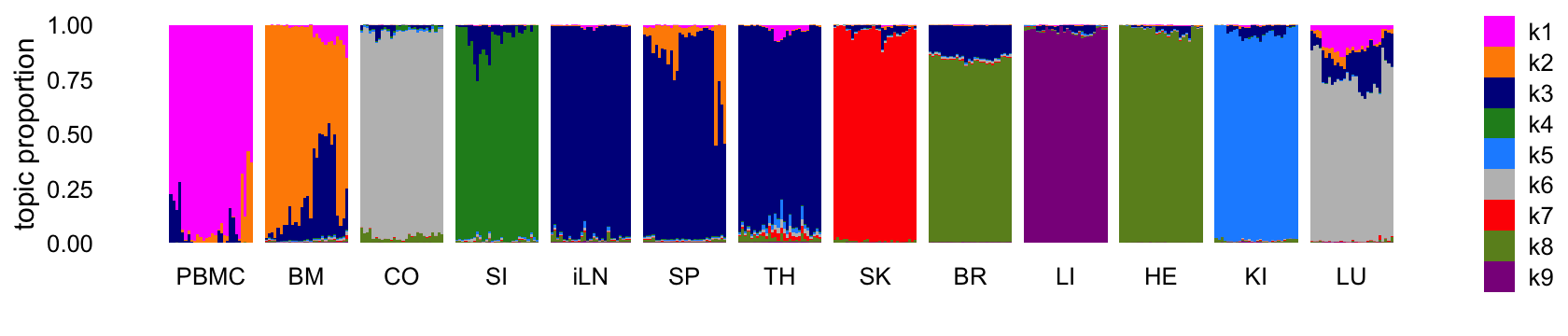
| Version | Author | Date |
|---|---|---|
| e558f17 | Peter Carbonetto | 2025-07-04 |
Abbreviations used: BM = bone marrow; BR = brain; CO = colon; HE = heart; iLN = inguinal lymph node; KI = kidney; LI = liver; LU = lung; SI = small intestine; SK = skin; SP = spleen; TH = thymus.
The topics largely correspond to the different tissues, although because there are more tissues than topics, some tissues that are more similar to each other shared the same topic. It is also interesting that, for the most part, none of the topics are capturing changes downstream of the LPS treatment. So presumably these expression changes are more subtle than the differences in expression among the tissues.
Fit a topic model with \(K = 14\) topics to the counts:
set.seed(1)
tm <- fit_poisson_nmf(counts,k = 14,init.method = "random",method = "em",
                      numiter = 20,verbose = "none",
                      control = list(numiter = 4,nc = 8,extrapolate = FALSE))
tm <- fit_poisson_nmf(counts,fit0 = tm,method = "scd",numiter = 40,
                      control = list(numiter = 4,nc = 8,extrapolate = TRUE),
                      verbose = "none")
Warning: The above code chunk cached its results, but
it won’t be re-run if previous chunks it depends on are updated. If you
need to use caching, it is highly recommended to also set
knitr::opts_chunk$set(autodep = TRUE) at the top of the
file (in a chunk that is not cached). Alternatively, you can customize
the option dependson for each individual chunk that is
cached. Using either autodep or dependson will
remove this warning. See the
knitr cache options for more details.
Structure plot comparing the topics to the tissue types:
structure_plot(tm,grouping = samples$tissue,gap = 4,
               topics = 1:14,colors = topic_colors,
               loadings_order = rows) +
  labs(fill = "") +
  theme(axis.text.x = element_text(angle = 0,hjust = 0.5),
        legend.key.height = unit(0.01,"cm"),
        legend.key.width = unit(0.2,"cm"),
        legend.text = element_text(size = 6))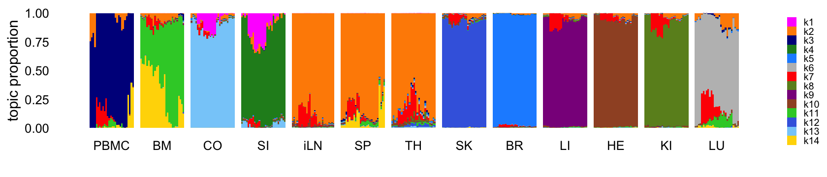
This next structure plot better highlights the topics that are capturing expression changes over time, some being presumably driven by the LPS-induced sepsis:
topic_colors <- c("magenta","gray50","gray65","gray40",
                  "gray85","gray75","red","gray80","gray90",
                  "gray60","limegreen","gray70","gray55",
                  "gold")
structure_plot(tm,grouping = samples$tissue,gap = 4,
               topics = 1:14,colors = topic_colors,
               loadings_order = rows) +
  labs(fill = "") +
  theme(axis.text.x = element_text(angle = 0,hjust = 0.5),
        legend.key.height = unit(0.01,"cm"),
        legend.key.width = unit(0.2,"cm"),
        legend.text = element_text(size = 6))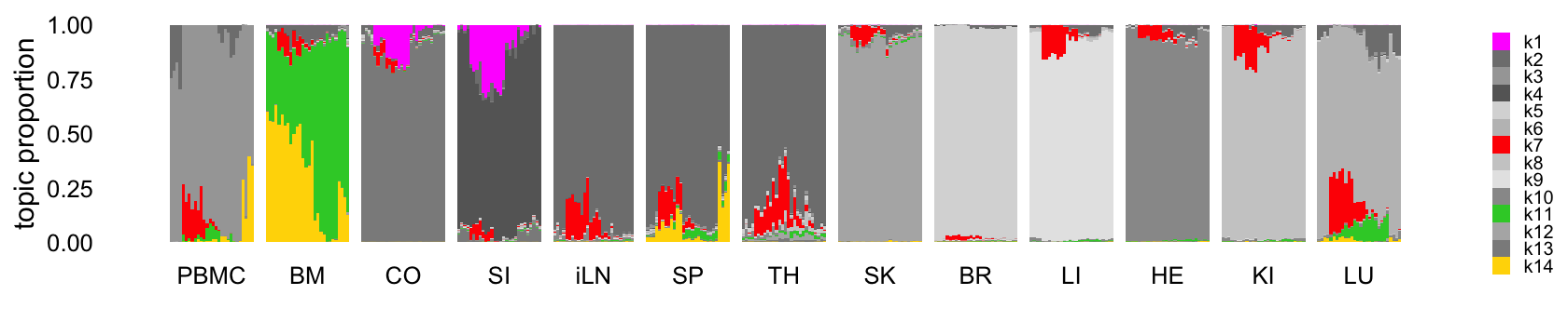
EBNMF (flashier)
Similar to the topic modeling analysis, let’s start by fitting an EBNMF to the shifted log counts using flashier, first with \(K = 9\). Since the greedy initialization does not seem to work well in this example, I’ll use a different initialization strategy: obtain a “good” initialization using the NNLM package, then use this initialization to fit a NMF using flashier. This approach is implemented in the following function:
Now fit an NMF to the shifted log counts, with \(K = 9\):
set.seed(1)
n  <- nrow(shifted_log_counts)
x  <- rpois(1e7,1/n)
s1 <- sd(log(x + 1))
set.seed(1)
fl_nmf_k9 <- flashier_nmf(shifted_log_counts,k = 9,greedy_init = TRUE,
                          var_type = 2,S = s1,verbose = 0)
Warning: The above code chunk cached its results, but
it won’t be re-run if previous chunks it depends on are updated. If you
need to use caching, it is highly recommended to also set
knitr::opts_chunk$set(autodep = TRUE) at the top of the
file (in a chunk that is not cached). Alternatively, you can customize
the option dependson for each individual chunk that is
cached. Using either autodep or dependson will
remove this warning. See the
knitr cache options for more details.
Structure plot comparing the topics to the tissue types:
rows <- order(samples$timepoint)
topic_colors <- c("powderblue","darkorange","olivedrab","limegreen",
                  "forestgreen","cyan","darkmagenta","gray","dodgerblue",
                  "red","gold","darkblue","lightskyblue",
                  "royalblue","sienna")
L <- ldf(fl_nmf_k9,type = "i")$L
structure_plot(L,grouping = samples$tissue,gap = 4,
               topics = 1:9,colors = topic_colors,
               loadings_order = rows) +
  labs(fill = "",y = "membership")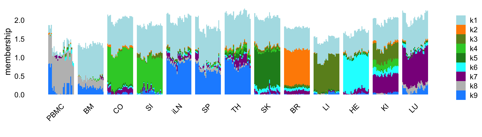
| Version | Author | Date |
|---|---|---|
| e558f17 | Peter Carbonetto | 2025-07-04 |
Like the topic model, the EBNMF model with \(K = 9\) does not capture any changes downstream of the LPS-induced sepsis.
Next fit an NMF to the shifted log counts using flashier, with \(K = 15\):
set.seed(1)
fl_nmf <- flashier_nmf(shifted_log_counts,k = 15,greedy_init = TRUE,
                       var_type = 2,S = s1,verbose = 0)
Warning: The above code chunk cached its results, but
it won’t be re-run if previous chunks it depends on are updated. If you
need to use caching, it is highly recommended to also set
knitr::opts_chunk$set(autodep = TRUE) at the top of the
file (in a chunk that is not cached). Alternatively, you can customize
the option dependson for each individual chunk that is
cached. Using either autodep or dependson will
remove this warning. See the
knitr cache options for more details.
Structure plot comparing the factors to the tissue types:
L <- ldf(fl_nmf,type = "i")$L
structure_plot(L,grouping = samples$tissue,gap = 4,
               topics = 1:15,colors = topic_colors,
               loadings_order = rows) +
  labs(fill = "",y = "membership") +
  theme(axis.text.x = element_text(angle = 0,hjust = 0.5),
        legend.key.height = unit(0.01,"cm"),
        legend.key.width = unit(0.25,"cm"),
        legend.text = element_text(size = 7))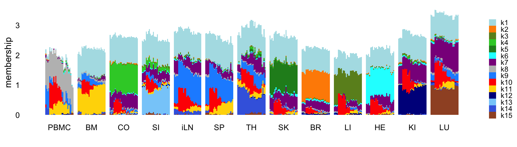
This next structure plot better highlights the topics that capture the processes that are driven or may be driven by LPS-induced sepsis:
rows <- order(samples$timepoint)
topic_colors <- c("gray95","gray70","gray80","gray50",
                  "gray60","gray90","gray75","gray","gray85",
                  "red","gold","gray65","gray45",
                  "gray35","gray75")
L <- ldf(fl_nmf,type = "i")$L
structure_plot(L,grouping = samples$tissue,gap = 4,
                    topics = 1:15,colors = topic_colors,
                    loadings_order = rows) +
  labs(fill = "",y = "membership") +
  theme(axis.text.x = element_text(angle = 0,hjust = 0.5),
        legend.key.height = unit(0.01,"cm"),
        legend.key.width = unit(0.25,"cm"),
        legend.text = element_text(size = 7))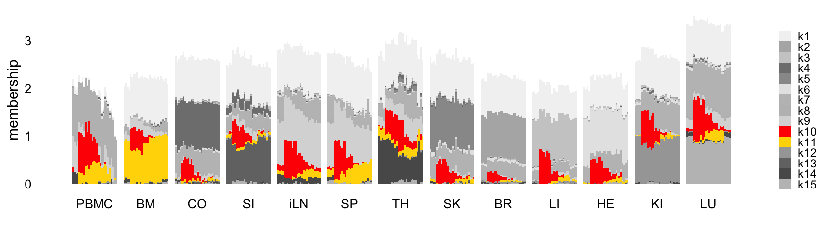
EBNMF with “cross-cutting” factor(s)
ADD TEXT HERE.
set.seed(1)
fl_nmf_cc <- flash_init(shifted_log_counts,S = s1,var_type = 2)
nn_factors <- c(1:9,12:15)
cc_factors <- 10:11
for (k in nn_factors) {
  l <- fl_nmf$L_pm[,k,drop = FALSE]
  f <- fl_nmf$F_pm[,k,drop = FALSE]
  fl_nmf_cc <- flash_factors_init(fl_nmf_cc,list(l,f),
                                  ebnm_fn = ebnm_point_exponential)
}
for (k in cc_factors) {
  l <- fl_nmf$L_pm[,k,drop = FALSE]
  f <- fl_nmf$F_pm[,k,drop = FALSE]
  fl_nmf_cc <- flash_factors_init(fl_nmf_cc,list(l,f),
                                  ebnm_fn = c(ebnm_point_exponential,
                                              ebnm_point_laplace))
}
fl_nmf_cc <- flash_backfit(fl_nmf_cc,extrapolate = FALSE,maxiter = 100,
                           verbose = 2)
fl_nmf_cc <- flash_backfit(fl_nmf_cc,extrapolate = TRUE,maxiter = 100,
                           verbose = 2)
Comparison with UMAP
Here I project the samples onto a 2-d embedding using UMAP to show that this LPS-related substructure is not obvious from a UMAP plot.
set.seed(1)
U <- rsvd(shifted_log_counts,k = 40)$u
Y <- umap(U,n_neighbors = 20,metric = "cosine",min_dist = 0.3,
          n_threads = 8,verbose = FALSE)
x <- Y[,1]
y <- Y[,2]
samples$umap1 <- x
samples$umap2 <- y
I color the samples in the UMAP plot by tissue (top-left) and by membership to factor 6 (top-right, bottom-left):
tissue_colors <- c("magenta","darkorange","darkblue","forestgreen",
                   "dodgerblue","red","olivedrab","darkmagenta",
                   "sienna","limegreen","royalblue","lightskyblue",
                   "gold")
L            <- ldf(fl_nmf,type = "i")$L
colnames(L)  <- paste0("k",1:15)
pdat         <- samples
pdat$factor6 <- L[,"k6"]
pdat$topic7  <- poisson2multinom(tm)$L[,"k7"]
p1 <- ggplot(pdat,aes(x = umap1,y = umap2,color = tissue)) +
  geom_point(size = 1) +
  scale_color_manual(values = tissue_colors) +
  theme_cowplot(font_size = 10)
p2 <- ggplot(pdat,aes(x = umap1,y = umap2,color = factor6)) +
  geom_point(size = 1) +
  scale_color_gradient2(low = "deepskyblue",mid = "gold",high = "tomato",
                        midpoint = 0.66) +
  theme_cowplot(font_size = 10)
p3 <- ggplot(pdat,aes(x = umap1,y = umap2,color = topic7)) +
  geom_point(size = 1) +
  scale_color_gradient2(low = "deepskyblue",mid = "gold",high = "tomato",
                        midpoint = 0.15) +
  theme_cowplot(font_size = 10)
plot_grid(p1,p2,p3,nrow = 2,ncol = 2)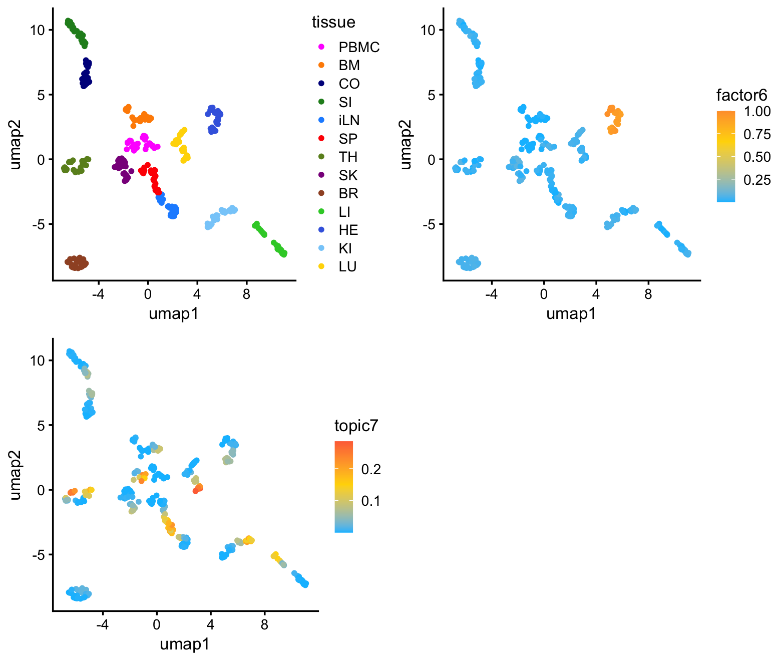
As expected, the predominant structure is due to the different tissues, with more similar tissues clustering together. There is also some more subtle structure within each cluster that appears to correspond well with factor 6 (and topic 7). So althought the UMAP does seem to reveal the sepsis-related structure, it cannot isolate the sepsis-related gene expression signature.
Factors isolating responses to LPS-induced sepsis
From the Structure plots, it appears that topic 7, and possibly topic 1, are capturing processes activated by LPS. However, I conjecture that it is difficult to determine which genes should members of topic 1 and which are members of the colon and small intensine topics. Indeed, topic 1 shares many genes with these two topics:
pdat <- cbind(data.frame(gene = colnames(counts)),
              poisson2multinom(tm)$F)
rows <- which(pdat$k1 < 0.01)
pdat[rows,"gene"] <- ""
p1 <- ggplot(pdat,aes(x = k1,y = k4,label = gene)) +
  geom_point() +
  geom_text_repel(color = "gray",size = 2.5,max.overlaps = Inf) +
  scale_x_continuous(trans = "sqrt") +
  scale_y_continuous(trans = "sqrt") +
  theme_cowplot(font_size = 10)
p2 <- ggplot(pdat,aes(x = k1,y = k13,label = gene)) +
  geom_point() +
  geom_text_repel(color = "gray",size = 2.5,max.overlaps = Inf) +
  scale_x_continuous(trans = "sqrt") +
  scale_y_continuous(trans = "sqrt") +
  theme_cowplot(font_size = 10)
plot_grid(p1,p2,nrow = 1,ncol = 2)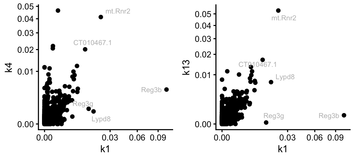
Still, it is interesting that three genes, Reg3b, Reg3g and Lypd8, stand out in topic 1 as distinct from the colon and SI topics. Let’s now contrast this to the situation for topic 7:
pdat <- cbind(data.frame(gene = colnames(counts)),
              poisson2multinom(tm)$F)
rows <- which(pdat$k7 < 0.008)
pdat[rows,"gene"] <- ""
p1 <- ggplot(pdat,aes(x = k7,y = k6,label = gene)) +
  geom_point() +
  geom_text_repel(color = "gray",size = 2.5,max.overlaps = Inf) +
  scale_x_continuous(trans = "sqrt") +
  scale_y_continuous(trans = "sqrt") +
  theme_cowplot(font_size = 10)
p2 <- ggplot(pdat,aes(x = k7,y = k8,label = gene)) +
  geom_point() +
  geom_text_repel(color = "gray",size = 2.5,max.overlaps = Inf) +
  scale_x_continuous(trans = "sqrt") +
  scale_y_continuous(trans = "sqrt") +
  theme_cowplot(font_size = 10)
plot_grid(p1,p2,nrow = 1,ncol = 2)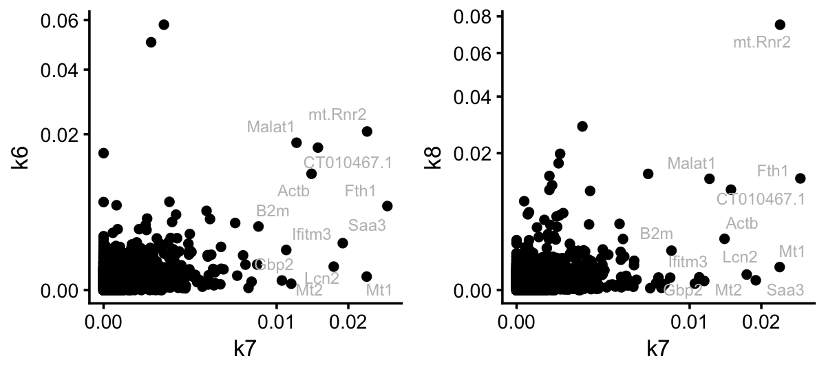
For illustration, I compared topic 7 to the kidney and lung topics. The key point here is that the topic model has selected genes for topic 7 that are very independent of the tissue topics. So this looks quite promising. Let’s now see if the result is similar for the EBNMF model fitted to the shifted log counts:
F <- ldf(fl_nmf,type = "i")$F
colnames(F) <- paste0("k",1:15)
pdat <- data.frame(tm   = poisson2multinom(tm)$F[,"k7"],
                   nmf  = F[,"k6"],
                   gene = rownames(F))
rows <- which(with(pdat,tm < 0.005 & nmf < 0.8))
pdat[rows,"gene"] <- ""
ggplot(pdat,aes(x = (tm)^(1/3),y = nmf,label = gene)) +
  geom_point() +
  geom_text_repel(color = "gray",size = 2.5,max.overlaps = Inf) +
  labs(x = "topic 7",y = "factor 6") +
  theme_cowplot(font_size = 12)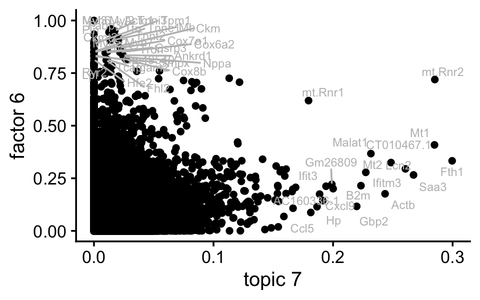
Indeed, factor 6 and topic 7 are cpaturing very similar expression patterns.
Next I ran GSEA on the on factor 6. (Running GSEA on topic 7 is complicated by the fact that it would be better to “shrink” the estimates before running GSEA, whereas this was automatically done for EBNMF result.)
data(gene_sets_mouse)
gene_sets     <- gene_sets_mouse$gene_sets
gene_info     <- gene_sets_mouse$gene_info
gene_set_info <- gene_sets_mouse$gene_set_info
j <- which(with(gene_sets_mouse$gene_set_info,
                (database == "MSigDB-C2" &
                 grepl("CP",sub_category_code,fixed = TRUE)) |
                (database == "MSigDB-C5") &
                 grepl("GO",sub_category_code,fixed = TRUE)))
genes <- sort(intersect(rownames(F),gene_info$Symbol))
i     <- which(is.element(gene_info$Symbol,genes))
gene_info     <- gene_info[i,]
gene_set_info <- gene_set_info[j,]
gene_sets     <- gene_sets[i,j]
rownames(gene_sets) <- gene_info$Symbol
rownames(gene_set_info) <- gene_set_info$id
gene_set_info <- gene_set_info[,-2]
F <- ldf(fl_nmf,type = "i")$F
colnames(F) <- paste0("k",1:15)
gsea_fl_nmf <- singlecelljamboreeR::perform_gsea(F[,"k6"],gene_sets,
                                                 gene_set_info,L = 15,
                                                 verbose = FALSE)
write.csv(data.frame(gene = rownames(F),signal = round(F[,"k6"],digits = 6)),
          "lps_fl_nmf_k6.csv",row.names = FALSE,quote = FALSE)
out <- gsea_fl_nmf$selected_gene_sets
out$top_genes <- sapply(out$top_genes,function (x) paste(x,collapse = " "))
out$lbf  <- round(out$lbf,digits = 6)
out$pip  <- round(out$pip,digits = 6)
out$coef <- round(out$coef,digits = 6)
write_csv(out,"lps_gsea_fl_nmf_k6.csv",quote = "none")
The top gene set is the IFN-\(\alpha/\beta\) signaling pathway, but other gene sets clearly relate to inflammation and immune system function:
print(gsea_fl_nmf$selected_gene_sets[c(2:7,9)],n = Inf)
# # A tibble: 15 × 7
#    CS    gene_set   lbf   pip   coef genes name
#    <fct> <chr>    <dbl> <dbl>  <dbl> <dbl> <chr>
#  1 L1    M516     488.  1     0.225    157 REACTOME_THE_CITRIC_ACID_TCA_CYCLE_A…
#  2 L2    M6298    193.  1     0.119    231 GO_CONTRACTILE_FIBER
#  3 L4    M24087   124.  1.000 0.129    130 GO_CARDIAC_MUSCLE_CONTRACTION
#  4 L7    M8229    112.  1     0.0830   287 REACTOME_TRANSLATION
#  5 L5    M13993   104.  1.000 0.0959   201 GO_CARDIAC_MUSCLE_TISSUE_DEVELOPMENT
#  6 L3    M17748   102.  1.000 0.0868   240 GO_MITOCHONDRIAL_PROTEIN_COMPLEX
#  7 L9    M23771    95.2 0.998 0.0780   280 GO_ATP_METABOLIC_PROCESS
#  8 L11   M39596    93.4 1     0.224     33 WP_FATTY_ACID_BETA_OXIDATION
#  9 L10   M17544    93.0 1     0.146     78 GO_SARCOPLASM
# 10 L14   M17675    80.2 1.000 0.198     37 GO_A_BAND
# 11 L13   M27932    80.2 1.000 0.0948   162 REACTOME_PROTEIN_LOCALIZATION
# 12 L8    M13855    67.3 1.000 0.0590   362 GO_POST_TRANSLATIONAL_PROTEIN_MODIFI…
# 13 L12   M13349    62.6 0.980 0.135     64 GO_MYOFIBRIL_ASSEMBLY
# 14 L15   M835      46.4 0.999 0.101     89 KEGG_DILATED_CARDIOMYOPATHY
# 15 L6    M11835    44.9 0.992 0.147     41 KEGG_VALINE_LEUCINE_AND_ISOLEUCINE_D…
This is the same scatterplot as the one just above, but with the genes in the IFN-\(\alpha/\beta\) signaling pathway highlighted:
pdat$pathway <- FALSE
pathway_genes <- names(which(gene_sets[,"M973"] > 0))
pdat[pathway_genes,"pathway"] <- TRUE
pdat <- pdat[order(pdat$pathway),]
ggplot(pdat,aes(x = (tm)^(1/3),y = nmf,label = gene,color = pathway)) +
  geom_point() +
  geom_text_repel(color = "gray",size = 2.5,max.overlaps = Inf) +
  scale_color_manual(values = c("darkblue","orangered")) +
  labs(x = "topic 7",y = "factor 6") +
  theme_cowplot(font_size = 12)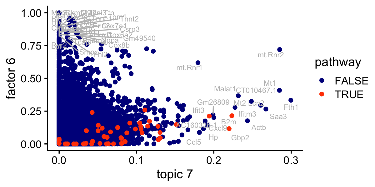
Here’s another view of the enrichment of the genes in the IFN-\(\alpha/\beta\) pathway:
p1 <- ggplot(subset(pdat,pathway),aes(x = nmf)) +
  geom_histogram(color = "white",fill = "black",bins = 16) +
  labs(x = "factor 6",y = "IFN-a/b genes") +
  theme_cowplot(font_size = 10)
p2 <- ggplot(subset(pdat,!pathway),aes(x = nmf)) +
  geom_histogram(color = "white",fill = "black",bins = 24) +
  labs(x = "factor 6",y = "other genes") +
  theme_cowplot(font_size = 10)
p3 <- ggplot(subset(pdat,pathway),aes(x = log10(tm + 1e-6))) +
  geom_histogram(color = "white",fill = "black",bins = 16) +
  labs(x = "topic 7",y = "IFN-a/b genes") +
  theme_cowplot(font_size = 10)
p4 <- ggplot(subset(pdat,!pathway),aes(x = log10(tm + 1e-6))) +
  geom_histogram(color = "white",fill = "black",bins = 24) +
  labs(x = "topic 7",y = "other genes") +
  theme_cowplot(font_size = 10)
plot_grid(p1,p2,p3,p4,nrow = 2,ncol = 2)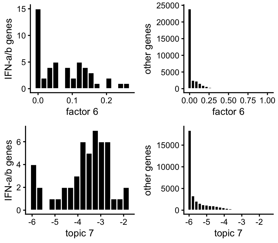
| Version | Author | Date |
|---|---|---|
| de50dc2 | Peter Carbonetto | 2025-07-17 |
sessionInfo()
# R version 4.3.3 (2024-02-29)
# Platform: aarch64-apple-darwin20 (64-bit)
# Running under: macOS 15.5
#
# Matrix products: default
# BLAS:   /Library/Frameworks/R.framework/Versions/4.3-arm64/Resources/lib/libRblas.0.dylib
# LAPACK: /Library/Frameworks/R.framework/Versions/4.3-arm64/Resources/lib/libRlapack.dylib;  LAPACK version 3.11.0
#
# locale:
# [1] en_US.UTF-8/en_US.UTF-8/en_US.UTF-8/C/en_US.UTF-8/en_US.UTF-8
#
# time zone: America/Chicago
# tzcode source: internal
#
# attached base packages:
# [1] stats     graphics  grDevices utils     datasets  methods   base
#
# other attached packages:
#  [1] uwot_0.2.3                 rsvd_1.0.5
#  [3] cowplot_1.1.3              ggrepel_0.9.6
#  [5] ggplot2_3.5.2              singlecelljamboreeR_0.1-36
#  [7] pathways_0.1-20            flashier_1.0.56
#  [9] ebnm_1.1-34                NNLM_0.4.4
# [11] fastTopics_0.7-25          data.table_1.17.6
# [13] readr_2.1.5                Matrix_1.6-5
#
# loaded via a namespace (and not attached):
#   [1] pbapply_1.7-2        rlang_1.1.6          magrittr_2.0.3
#   [4] git2r_0.33.0         RcppAnnoy_0.0.22     horseshoe_0.2.0
#   [7] matrixStats_1.2.0    susieR_0.14.6        compiler_4.3.3
#  [10] vctrs_0.6.5          reshape2_1.4.4       RcppZiggurat_0.1.6
#  [13] quadprog_1.5-8       stringr_1.5.1        pkgconfig_2.0.3
#  [16] crayon_1.5.3         fastmap_1.2.0        labeling_0.4.3
#  [19] utf8_1.2.6           promises_1.3.3       rmarkdown_2.29
#  [22] tzdb_0.4.0           bit_4.0.5            purrr_1.0.4
#  [25] Rfast_2.1.0          xfun_0.52            cachem_1.1.0
#  [28] trust_0.1-8          jsonlite_2.0.0       progress_1.2.3
#  [31] later_1.4.2          reshape_0.8.9        BiocParallel_1.36.0
#  [34] irlba_2.3.5.1        parallel_4.3.3       prettyunits_1.2.0
#  [37] R6_2.6.1             bslib_0.9.0          stringi_1.8.7
#  [40] RColorBrewer_1.1-3   SQUAREM_2021.1       jquerylib_0.1.4
#  [43] Rcpp_1.1.0           knitr_1.50           R.utils_2.12.3
#  [46] httpuv_1.6.14        splines_4.3.3        tidyselect_1.2.1
#  [49] dichromat_2.0-0.1    yaml_2.3.10          codetools_0.2-19
#  [52] lattice_0.22-5       tibble_3.3.0         plyr_1.8.9
#  [55] withr_3.0.2          evaluate_1.0.4       Rtsne_0.17
#  [58] RcppParallel_5.1.10  pillar_1.11.0        whisker_0.4.1
#  [61] plotly_4.11.0        softImpute_1.4-3     generics_0.1.4
#  [64] vroom_1.6.5          rprojroot_2.0.4      invgamma_1.2
#  [67] truncnorm_1.0-9      hms_1.1.3            scales_1.4.0
#  [70] ashr_2.2-66          gtools_3.9.5         RhpcBLASctl_0.23-42
#  [73] glue_1.8.0           scatterplot3d_0.3-44 lazyeval_0.2.2
#  [76] tools_4.3.3          fgsea_1.35.4         fs_1.6.6
#  [79] fastmatch_1.1-6      grid_4.3.3           tidyr_1.3.1
#  [82] colorspace_2.1-0     deconvolveR_1.2-1    cli_3.6.5
#  [85] Polychrome_1.5.1     workflowr_1.7.1      mixsqp_0.3-54
#  [88] viridisLite_0.4.2    dplyr_1.1.4          gtable_0.3.6
#  [91] R.methodsS3_1.8.2    sass_0.4.10          digest_0.6.37
#  [94] htmlwidgets_1.6.4    farver_2.1.2         R.oo_1.26.0
#  [97] htmltools_0.5.8.1    lifecycle_1.0.4      httr_1.4.7
# [100] bit64_4.0.5