Initial exploration of the pancreas data set
Peter Carbonetto
Last updated: 2024-10-31
Checks: 7 0
Knit directory:
single-cell-jamboree/analysis/
This reproducible R Markdown analysis was created with workflowr (version 1.7.1). The Checks tab describes the reproducibility checks that were applied when the results were created. The Past versions tab lists the development history.
Great! Since the R Markdown file has been committed to the Git repository, you know the exact version of the code that produced these results.
Great job! The global environment was empty. Objects defined in the global environment can affect the analysis in your R Markdown file in unknown ways. For reproduciblity it’s best to always run the code in an empty environment.
The command set.seed(1) was run prior to running the
code in the R Markdown file. Setting a seed ensures that any results
that rely on randomness, e.g. subsampling or permutations, are
reproducible.
Great job! Recording the operating system, R version, and package versions is critical for reproducibility.
Nice! There were no cached chunks for this analysis, so you can be confident that you successfully produced the results during this run.
Great job! Using relative paths to the files within your workflowr project makes it easier to run your code on other machines.
Great! You are using Git for version control. Tracking code development and connecting the code version to the results is critical for reproducibility.
The results in this page were generated with repository version 886cd01. See the Past versions tab to see a history of the changes made to the R Markdown and HTML files.
Note that you need to be careful to ensure that all relevant files for
the analysis have been committed to Git prior to generating the results
(you can use wflow_publish or
wflow_git_commit). workflowr only checks the R Markdown
file, but you know if there are other scripts or data files that it
depends on. Below is the status of the Git repository when the results
were generated:
Untracked files:
    Untracked:  analysis/pancreas.RData
    Untracked:  data/Immune_ALL_human.h5ad
    Untracked:  data/human_pancreas_norm_complexBatch.h5ad
Note that any generated files, e.g. HTML, png, CSS, etc., are not included in this status report because it is ok for generated content to have uncommitted changes.
These are the previous versions of the repository in which changes were
made to the R Markdown (analysis/pancreas.Rmd) and HTML
(docs/pancreas.html) files. If you’ve configured a remote
Git repository (see ?wflow_git_remote), click on the
hyperlinks in the table below to view the files as they were in that
past version.
| File | Version | Author | Date | Message |
|---|---|---|---|---|
| Rmd | 886cd01 | Peter Carbonetto | 2024-10-31 | workflowr::wflow_publish("pancreas.Rmd", verbose = TRUE, view = FALSE) |
| html | 528d5ef | Peter Carbonetto | 2024-10-30 | First build of the pancreas workflowr page. |
| Rmd | a1d7a17 | Peter Carbonetto | 2024-10-30 | Added some background on the pancreas data set. |
| Rmd | 3fa28da | Peter Carbonetto | 2024-10-30 | Small edit to pancreas.Rmd. |
| Rmd | 370a336 | Peter Carbonetto | 2024-10-30 | Still working on pancreas.Rmd. |
| Rmd | fbe0b62 | Peter Carbonetto | 2024-10-30 | Made a few improvements to the pancreas analysis. |
| Rmd | c090d1d | Peter Carbonetto | 2024-10-30 | Working on initial examination of pancreas data. |
The aim of this analysis is to take an initial look at the “pancreas” data set that was featured in in the Luecken et al 2022 benchmarking paper, and prepare the data in a convenient form for subsequent analyses in R.
In addition to being featured in the Luecken et al paper, it has been used in several papers on “data integration” methods for single-cell data (also known as “batch correction” or “harmonization” methods). See for example the MNN paper. The Supplementary Note in the Luecken et al paper has additional references.
See Supplementary Fig. 13, Supplementary Note 3 and Supplementary Data 7 of the Luecken et al paper for more information on this data set.
First, load the packages needed for this analysis.
library(tools)
library(Matrix)
library(MatrixExtra)
library(hdf5r)
library(uwot)
library(ggplot2)
library(cowplot)
Download the file “human_pancreas_norm_complexBatch.h5ad” from figshare and copy it to the “data” subdirectory of this git repository. Then load the count data, and encode them as a sparse matrix:
dat <- H5File$new("../data/human_pancreas_norm_complexBatch.h5ad",mode = "r")
counts <- dat[["layers"]][["counts"]][,]
counts <- as(counts,"CsparseMatrix")
counts <- t(counts)
sample_info <- data.frame(id          = dat[["obs"]][["_index"]][],
                          tech        = dat[["obs"]][["tech"]][],
                          celltype    = dat[["obs"]][["celltype"]][],
                          size_factor = dat[["obs"]][["size_factors"]][],
                          stringsAsFactors = FALSE)
sample_info <- transform(sample_info,
                         tech     = factor(tech),
                         celltype = factor(celltype))
levels(sample_info$tech)     <- dat[["obs"]][["__categories"]][["tech"]][]
levels(sample_info$celltype) <- dat[["obs"]][["__categories"]][["celltype"]][]
genes <- dat[["var"]][["_index"]][]
rownames(counts) <- sample_info$id
colnames(counts) <- genes
Note that some of the data are not actually counts, so perhaps calling this matrix “counts” is a bit misleading. Also note that in Luecken et al the counts were log-transformed, but here we taking the untransformed counts.
The matrix has 16,382 rows (cells) and 19,093 columns (genes), and about 18% of the entries are nonzeros:
nrow(counts)
ncol(counts)
mean(counts > 0)
# [1] 16382
# [1] 19093
# [1] 0.1779012
The pancreas data are actually several scRNA-seq data sets that were combined together:
table(sample_info$tech)
#
#     celseq    celseq2 fluidigmc1    inDrop1    inDrop2    inDrop3    inDrop4
#       1004       2285        638       1937       1724       3605       1303
#    smarter  smartseq2
#       1492       2394
The cells were previous annotated by cell type:
table(sample_info$celltype)
#
#             acinar activated_stellate              alpha               beta
#               1669                464               5493               4169
#              delta             ductal        endothelial            epsilon
#               1055               2142                313                 32
#              gamma         macrophage               mast quiescent_stellate
#                699                 79                 42                193
#            schwann             t_cell
#                 25                  7
Some of the cell types occur in only a very small number of cells.
Distribution of the size factors:
s <- rowSums(counts)
ggplot(data.frame(log_size_factor = log10(s)),aes(log_size_factor)) +
  geom_histogram(bins = 64,col = "black",fill = "black") +
  theme_cowplot(font_size = 10)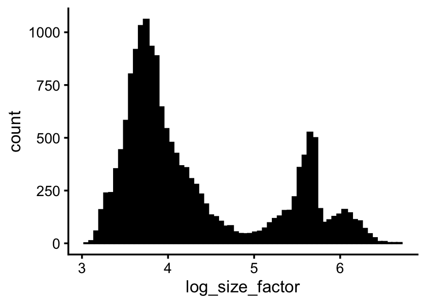
Genes with nonzero expression:
p <- colSums(counts)/sum(s)
sum(p > 0)
# [1] 18771
Distribution of the (relative) expression levels:
p <- p[p > 0]
ggplot(data.frame(log_rel_expression_level = log10(p)),
                  aes(log_rel_expression_level)) +
  geom_histogram(bins = 64,col = "black",fill = "black") +
  theme_cowplot(font_size = 10)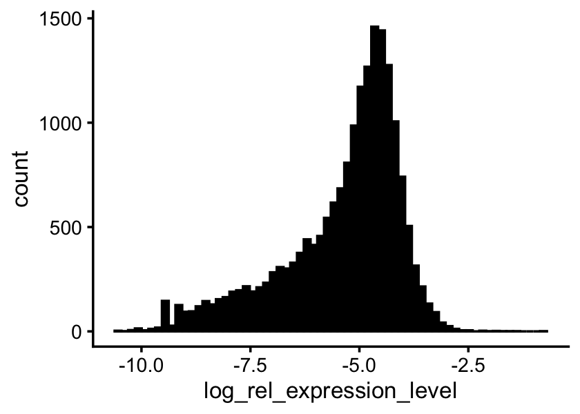
Now do UMAP… Compute the shifted log counts:
a <- 1
s <- rowSums(counts)
s <- s/mean(s)
Y <- mapSparse(counts/(a*s),log1p)
UMAP:
res <- umap(as.matrix(Y),n_components = 2,n_threads = 8,verbose = TRUE)TO DO: Save the data in an .Rdata file for more convenient analysis with the matrix factorization methods.
save(list = c("sample_info","counts"),file = "pancreas.RData")
resaveRdaFiles("pancreas.RData")
sessionInfo()
# R version 4.3.3 (2024-02-29)
# Platform: aarch64-apple-darwin20 (64-bit)
# Running under: macOS Sonoma 14.6.1
#
# Matrix products: default
# BLAS:   /Library/Frameworks/R.framework/Versions/4.3-arm64/Resources/lib/libRblas.0.dylib
# LAPACK: /Library/Frameworks/R.framework/Versions/4.3-arm64/Resources/lib/libRlapack.dylib;  LAPACK version 3.11.0
#
# locale:
# [1] en_US.UTF-8/en_US.UTF-8/en_US.UTF-8/C/en_US.UTF-8/en_US.UTF-8
#
# time zone: America/Chicago
# tzcode source: internal
#
# attached base packages:
# [1] tools     stats     graphics  grDevices utils     datasets  methods
# [8] base
#
# other attached packages:
# [1] cowplot_1.1.3      ggplot2_3.5.0      uwot_0.1.16        hdf5r_1.3.11
# [5] MatrixExtra_0.1.15 Matrix_1.6-5
#
# loaded via a namespace (and not attached):
#  [1] sass_0.4.8          utf8_1.2.4          generics_0.1.3
#  [4] stringi_1.8.3       lattice_0.22-5      digest_0.6.34
#  [7] magrittr_2.0.3      evaluate_0.23       grid_4.3.3
# [10] float_0.3-2         fastmap_1.1.1       rprojroot_2.0.4
# [13] workflowr_1.7.1     jsonlite_1.8.8      whisker_0.4.1
# [16] promises_1.2.1      fansi_1.0.6         scales_1.3.0
# [19] RhpcBLASctl_0.23-42 jquerylib_0.1.4     cli_3.6.2
# [22] rlang_1.1.3         bit64_4.0.5         munsell_0.5.0
# [25] withr_3.0.0         cachem_1.0.8        yaml_2.3.8
# [28] parallel_4.3.3      dplyr_1.1.4         colorspace_2.1-0
# [31] httpuv_1.6.14       vctrs_0.6.5         R6_2.5.1
# [34] lifecycle_1.0.4     git2r_0.33.0        stringr_1.5.1
# [37] fs_1.6.3            bit_4.0.5           pkgconfig_2.0.3
# [40] pillar_1.9.0        bslib_0.6.1         later_1.3.2
# [43] gtable_0.3.4        glue_1.7.0          Rcpp_1.0.12
# [46] highr_0.10          xfun_0.42           tibble_3.2.1
# [49] tidyselect_1.2.1    knitr_1.45          farver_2.1.1
# [52] htmltools_0.5.7     labeling_0.4.3      rmarkdown_2.26
# [55] compiler_4.3.3