Examine B-cell and NK cell topics and clusters
Peter Carbonetto
Last updated: 2020-09-08
Checks: 6 1
Knit directory: single-cell-topics/analysis/
This reproducible R Markdown analysis was created with workflowr (version 1.6.2.9000). The Checks tab describes the reproducibility checks that were applied when the results were created. The Past versions tab lists the development history.
Great! Since the R Markdown file has been committed to the Git repository, you know the exact version of the code that produced these results.
Great job! The global environment was empty. Objects defined in the global environment can affect the analysis in your R Markdown file in unknown ways. For reproduciblity it’s best to always run the code in an empty environment.
The command set.seed(1) was run prior to running the code in the R Markdown file. Setting a seed ensures that any results that rely on randomness, e.g. subsampling or permutations, are reproducible.
Great job! Recording the operating system, R version, and package versions is critical for reproducibility.
- diff-count-analysis-clusters-68k
- diff-count-analysis-clusters-purified
To ensure reproducibility of the results, delete the cache directory bcells_and_nkcells_cache and re-run the analysis. To have workflowr automatically delete the cache directory prior to building the file, set delete_cache = TRUE when running wflow_build() or wflow_publish().
Great job! Using relative paths to the files within your workflowr project makes it easier to run your code on other machines.
Great! You are using Git for version control. Tracking code development and connecting the code version to the results is critical for reproducibility.
The results in this page were generated with repository version 4525eda. See the Past versions tab to see a history of the changes made to the R Markdown and HTML files.
Note that you need to be careful to ensure that all relevant files for the analysis have been committed to Git prior to generating the results (you can use wflow_publish or wflow_git_commit). workflowr only checks the R Markdown file, but you know if there are other scripts or data files that it depends on. Below is the status of the Git repository when the results were generated:
Ignored files:
    Ignored:    data/droplet.RData
    Ignored:    data/pbmc_68k.RData
    Ignored:    data/pbmc_purified.RData
    Ignored:    data/pulseseq.RData
    Ignored:    output/droplet/fits-droplet.RData
    Ignored:    output/droplet/rds/
    Ignored:    output/pbmc-68k/fits-pbmc-68k.RData
    Ignored:    output/pbmc-68k/postfit-pbmc-68k-scd-ex-k=6.RData
    Ignored:    output/pbmc-68k/rds/
    Ignored:    output/pbmc-purified/fits-pbmc-purified.RData
    Ignored:    output/pbmc-purified/postfit-pbmc-purified-scd-ex-k=6.RData
    Ignored:    output/pbmc-purified/rds/
    Ignored:    output/pulseseq/fits-pulseseq.RData
    Ignored:    output/pulseseq/rds/

Untracked files:
    Untracked:  analysis/bcells_and_nkcells_cache/
Note that any generated files, e.g. HTML, png, CSS, etc., are not included in this status report because it is ok for generated content to have uncommitted changes.
These are the previous versions of the repository in which changes were made to the R Markdown (analysis/bcells_and_nkcells.Rmd) and HTML (docs/bcells_and_nkcells.html) files. If you’ve configured a remote Git repository (see ?wflow_git_remote), click on the hyperlinks in the table below to view the files as they were in that past version.
| File | Version | Author | Date | Message |
|---|---|---|---|---|
| Rmd | 4525eda | Peter Carbonetto | 2020-09-08 | workflowr::wflow_publish(“bcells_and_nkcells.Rmd”) |
| html | 2e5917d | Peter Carbonetto | 2020-09-08 | Performed first build of bcells_and_nkcells page. |
| Rmd | faea79b | Peter Carbonetto | 2020-09-08 | workflowr::wflow_publish(“bcells_and_nkcells.Rmd”) |
| Rmd | 681efe3 | Peter Carbonetto | 2020-09-08 | Added steps to bcells_and_nkcells analysis to run cluster-based differential expression analysis. |
| Rmd | 77499e2 | Peter Carbonetto | 2020-09-07 | Implemented first steps of bcells_and_nkcells analysis. |
| Rmd | d749c17 | Peter Carbonetto | 2020-09-07 | Added notes to plots_pbmc; committed pbmc-clustering.RData output. |
Add text here.
Load the packages used in the analysis below.
library(Matrix)
library(fastTopics)
library(ggplot2)
library(ggrepel)
library(cowplot)
source("../code/more_plots.R")
Load the mixture of FACS-purified PBMC data, the \(k = 6\) Poisson NMF model fit, and the results of the differential expression analysis using this model fit.
fit_purified <-
  readRDS("../output/pbmc-purified/rds/fit-pbmc-purified-scd-ex-k=6.rds")$fit
load("../output/pbmc-purified/postfit-pbmc-purified-scd-ex-k=6.RData")
load("../data/pbmc_purified.RData")
ids                 <- rownames(diff_count_res$Z)
counts_purified     <- counts[,ids]
genes_purified      <- genes[match(ids,genes$ensembl),]
diff_count_purified <- diff_count_res
rm(samples,genes,counts,diff_count_res,gene_info,ids)
rm(gene_set_info,gene_sets,gsea_res)
Load the “unsorted” 68k PBMC data, the \(k = 6\) Poisson NMF model fit, and the results of the differential expression analysis using this model fit.
fit_68k <- readRDS("../output/pbmc-68k/rds/fit-pbmc-68k-scd-ex-k=6.rds")$fit
load("../output/pbmc-68k/postfit-pbmc-68k-scd-ex-k=6.RData")
load("../data/pbmc_68k.RData")
ids            <- rownames(diff_count_res$Z)
counts_68k     <- counts[,ids]
genes_68k      <- genes[match(ids,genes$ensembl),]
diff_count_68k <- diff_count_res
rm(samples,genes,counts,diff_count_res,ids,gene_set_info,gene_sets,gsea_res)
Load the clustering of the purified and 68k data set that was determined in the “plots_pbmc” analysis.
load("../output/pbmc-clustering.RData")Perform a differential expression analysis using the clustering of the purified data.
fit_clusters_purified <-
  init_poisson_nmf_from_clustering(counts_purified,samples_purified$cluster)
diff_count_clusters_purified <- diff_count_analysis(fit_clusters_purified,
                                                    counts_purified)
# All topic proportions are either zero or one; using simpler single-topic calculations for model parameter estimates
# Fitting 17316 x 6 = 103896 univariate Poisson models.
# Computing log-fold change statistics.
Warning: The above code chunk cached its results, but it won’t be re-run if previous chunks it depends on are updated. If you need to use caching, it is highly recommended to also set knitr::opts_chunk$set(autodep = TRUE) at the top of the file (in a chunk that is not cached). Alternatively, you can customize the option dependson for each individual chunk that is cached. Using either autodep or dependson will remove this warning. See the knitr cache options for more details.
Perform a differential expression analysis using the clustering of the 68k data.
fit_clusters_68k <- init_poisson_nmf_from_clustering(counts_68k,
                                                     samples_68k$cluster)
diff_count_clusters_68k <- diff_count_analysis(fit_clusters_68k,counts_68k)
# All topic proportions are either zero or one; using simpler single-topic calculations for model parameter estimates
# Fitting 16402 x 9 = 147618 univariate Poisson models.
# Computing log-fold change statistics.
Warning: The above code chunk cached its results, but it won’t be re-run if previous chunks it depends on are updated. If you need to use caching, it is highly recommended to also set knitr::opts_chunk$set(autodep = TRUE) at the top of the file (in a chunk that is not cached). Alternatively, you can customize the option dependson for each individual chunk that is cached. Using either autodep or dependson will remove this warning. See the knitr cache options for more details.
In the purified data set, compare the gene-wise z-scores from topic 3 to the \(z\)-scores from cluster B.
p1 <- diff_count_scatterplot(diff_count_clusters_purified$Z[,"B"],
                             diff_count_purified$Z[,3],
                             diff_count_purified$colmeans,
                             genes_purified$symbol,
                             label_above_score = 100) +
  labs(x = "cluster B",y = "topic 3",title = "z-scores")
print(p1)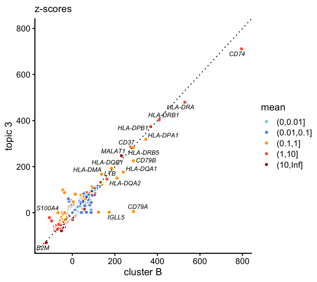
In the 68k data, compare the gene-wise z-scores from topic 5 to the \(z\)-scores from cluster A2.
p2 <- diff_count_scatterplot(diff_count_clusters_68k$Z[,"A2"],
                             diff_count_68k$Z[,5],
                             diff_count_68k$colmeans,
                             genes_68k$symbol,
                             label_above_score = 100) +
  labs(x = "cluster A2",y = "topic 5",title = "z-scores")
print(p2)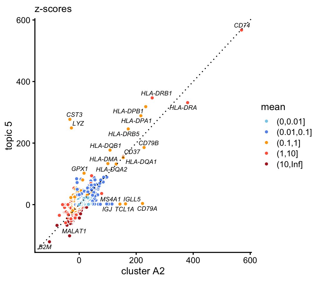
| Version | Author | Date |
|---|---|---|
| 2e5917d | Peter Carbonetto | 2020-09-08 |
Plot histograms of the topic 3 proportions inside and outside cluster B in the purified data.
fit <- poisson2multinom(fit_purified)
p3 <- ggplot(data.frame(x = fit$L[,3]),aes(x)) +
  geom_histogram(bins = 50,color = "white",fill = "black",na.rm = TRUE) +
  ylim(c(0,2000)) +
  labs(x = "topic 3 proportion",y = "number of cells") +
  theme_cowplot(font_size = 10)
p4 <- ggplot(data.frame(x = fit$L[samples_purified$cluster == "B",3]),aes(x)) +
  geom_histogram(bins = 30,color = "white",fill = "black",na.rm = TRUE) +
  labs(x = "topic 3 proportion",y = "number of cells") +
  theme_cowplot(font_size = 10)
plot_grid(p3,p4)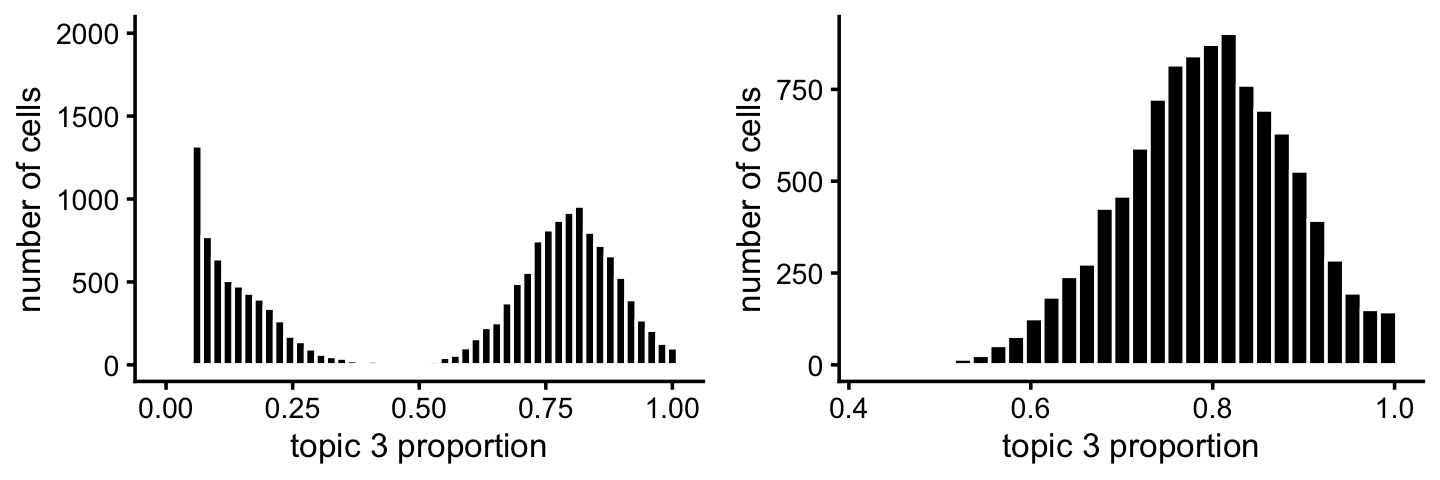
Plot histograms of the topic 5 proportions inside and outside cluster A3 in the 68k data.
fit <- poisson2multinom(fit_68k)
p5 <- ggplot(data.frame(x = fit$L[,5]),aes(x)) +
  geom_histogram(bins = 50,color = "white",fill = "black",na.rm = TRUE) +
  ylim(c(0,1200)) +
  labs(x = "topic 5 proportion",y = "number of cells") +
  theme_cowplot(font_size = 10)
p6 <- ggplot(data.frame(x = fit$L[samples_68k$cluster == "A2",5]),aes(x)) +
  geom_histogram(bins = 30,color = "white",fill = "black",na.rm = TRUE) +
  labs(x = "topic 5 proportion",y = "number of cells") +
  theme_cowplot(font_size = 10)
plot_grid(p5,p6)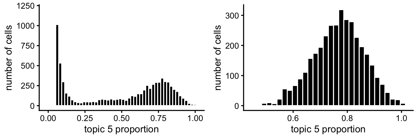
sessionInfo()
# R version 3.6.2 (2019-12-12)
# Platform: x86_64-apple-darwin15.6.0 (64-bit)
# Running under: macOS Catalina 10.15.6
#
# Matrix products: default
# BLAS:   /Library/Frameworks/R.framework/Versions/3.6/Resources/lib/libRblas.0.dylib
# LAPACK: /Library/Frameworks/R.framework/Versions/3.6/Resources/lib/libRlapack.dylib
#
# locale:
# [1] en_US.UTF-8/en_US.UTF-8/en_US.UTF-8/C/en_US.UTF-8/en_US.UTF-8
#
# attached base packages:
# [1] stats     graphics  grDevices utils     datasets  methods   base
#
# other attached packages:
# [1] cowplot_1.0.0      ggrepel_0.9.0      ggplot2_3.3.0      fastTopics_0.3-174
# [5] Matrix_1.2-18
#
# loaded via a namespace (and not attached):
#  [1] Rcpp_1.0.5           lattice_0.20-38      tidyr_1.0.0
#  [4] prettyunits_1.1.1    assertthat_0.2.1     zeallot_0.1.0
#  [7] rprojroot_1.3-2      digest_0.6.23        R6_2.4.1
# [10] backports_1.1.5      MatrixModels_0.4-1   evaluate_0.14
# [13] coda_0.19-3          httr_1.4.1           pillar_1.4.3
# [16] rlang_0.4.5          progress_1.2.2       lazyeval_0.2.2
# [19] data.table_1.12.8    irlba_2.3.3          SparseM_1.78
# [22] whisker_0.4          rmarkdown_2.3        labeling_0.3
# [25] Rtsne_0.15           stringr_1.4.0        htmlwidgets_1.5.1
# [28] munsell_0.5.0        compiler_3.6.2       httpuv_1.5.2
# [31] xfun_0.11            pkgconfig_2.0.3      mcmc_0.9-6
# [34] htmltools_0.4.0      tidyselect_0.2.5     tibble_2.1.3
# [37] workflowr_1.6.2.9000 quadprog_1.5-8       viridisLite_0.3.0
# [40] crayon_1.3.4         dplyr_0.8.3          withr_2.1.2
# [43] later_1.0.0          MASS_7.3-51.4        grid_3.6.2
# [46] jsonlite_1.6         gtable_0.3.0         lifecycle_0.1.0
# [49] git2r_0.26.1         magrittr_1.5         scales_1.1.0
# [52] RcppParallel_4.4.2   stringi_1.4.3        farver_2.0.1
# [55] fs_1.3.1             promises_1.1.0       vctrs_0.2.1
# [58] tools_3.6.2          glue_1.3.1           purrr_0.3.3
# [61] hms_0.5.2            yaml_2.2.0           colorspace_1.4-1
# [64] plotly_4.9.2         knitr_1.26           quantreg_5.54
# [67] MCMCpack_1.4-5