Differential expression analysis using a topic model: illustration in mixture of FACS-purified PBMC data
Peter Carbonetto
Last updated: 2021-11-21
Checks: 7 0
Knit directory: single-cell-topics/analysis/
This reproducible R Markdown analysis was created with workflowr (version 1.6.2). The Checks tab describes the reproducibility checks that were applied when the results were created. The Past versions tab lists the development history.
Great! Since the R Markdown file has been committed to the Git repository, you know the exact version of the code that produced these results.
Great job! The global environment was empty. Objects defined in the global environment can affect the analysis in your R Markdown file in unknown ways. For reproduciblity it’s best to always run the code in an empty environment.
The command set.seed(1) was run prior to running the code in the R Markdown file. Setting a seed ensures that any results that rely on randomness, e.g. subsampling or permutations, are reproducible.
Great job! Recording the operating system, R version, and package versions is critical for reproducibility.
Nice! There were no cached chunks for this analysis, so you can be confident that you successfully produced the results during this run.
Great job! Using relative paths to the files within your workflowr project makes it easier to run your code on other machines.
Great! You are using Git for version control. Tracking code development and connecting the code version to the results is critical for reproducibility.
The results in this page were generated with repository version f7a5a86. See the Past versions tab to see a history of the changes made to the R Markdown and HTML files.
Note that you need to be careful to ensure that all relevant files for the analysis have been committed to Git prior to generating the results (you can use wflow_publish or wflow_git_commit). workflowr only checks the R Markdown file, but you know if there are other scripts or data files that it depends on. Below is the status of the Git repository when the results were generated:
Ignored files:
    Ignored:    data/droplet.RData
    Ignored:    data/pbmc_68k.RData
    Ignored:    data/pbmc_purified.RData
    Ignored:    data/pulseseq.RData
    Ignored:    output/droplet/diff-count-droplet.RData
    Ignored:    output/droplet/fits-droplet.RData
    Ignored:    output/droplet/rds/
    Ignored:    output/pbmc-68k/fits-pbmc-68k.RData
    Ignored:    output/pbmc-68k/rds/
    Ignored:    output/pbmc-purified/fits-pbmc-purified.RData
    Ignored:    output/pbmc-purified/rds/
    Ignored:    output/pulseseq/diff-count-pulseseq.RData
    Ignored:    output/pulseseq/fits-pulseseq.RData
    Ignored:    output/pulseseq/rds/

Untracked files:
    Untracked:  analysis/de_analysis_detailed_look_cache/
    Untracked:  analysis/de_analysis_detailed_look_more_cache/
    Untracked:  plots/

Unstaged changes:
    Modified:   analysis/de_analysis_detailed_look.Rmd
    Modified:   analysis/temp6.R
Note that any generated files, e.g. HTML, png, CSS, etc., are not included in this status report because it is ok for generated content to have uncommitted changes.
These are the previous versions of the repository in which changes were made to the R Markdown (analysis/de_analysis_purified_pbmc.Rmd) and HTML (docs/de_analysis_purified_pbmc.html) files. If you’ve configured a remote Git repository (see ?wflow_git_remote), click on the hyperlinks in the table below to view the files as they were in that past version.
| File | Version | Author | Date | Message |
|---|---|---|---|---|
| Rmd | f7a5a86 | Peter Carbonetto | 2021-11-21 | workflowr::wflow_publish(“de_analysis_purified_pbmc.Rmd”) |
| html | 1917832 | Peter Carbonetto | 2021-11-21 | Working on de_analysis_purified_pbmc analysis. |
| Rmd | 90c6584 | Peter Carbonetto | 2021-11-21 | workflowr::wflow_publish(“de_analysis_purified_pbmc.Rmd”, verbose = TRUE) |
| Rmd | 3143481 | Peter Carbonetto | 2021-11-21 | Working on the de_analysis_purified_pbmc analysis. |
| Rmd | a16fdf9 | Peter Carbonetto | 2021-11-20 | Added structure plot to de_analysis_purified_pbmc analysis. |
| html | e1ab3a0 | Peter Carbonetto | 2021-11-08 | Built the initial de_analysis_purified_pbmc analysis page. |
| html | 2befadb | Peter Carbonetto | 2021-11-08 | Added link to overview page. |
| Rmd | 71e267d | Peter Carbonetto | 2021-11-08 | workflowr::wflow_publish(“index.Rmd”) |
The aim of this analysis is to understand the differences between a classical differential expresion analysis comparing expression among cell types (implemented using DESEq2) and a differential expression analysis using the topic model, which allows for grades of membership to cell types or cell states.
Begin by loading the packages and some function definitions used in the analysis.
library(Matrix)
library(fastTopics)
library(ggplot2)
library(cowplot)
source("../code/de_analysis_functions.R")
Load the UMI gene count data.
load("../data/pbmc_purified.RData")Load the \(K = 6\) Poisson NMF model fit, and convert it to a topic model.
fit <- readRDS(file.path("../output/pbmc-purified/rds",
                         "fit-pbmc-purified-scd-ex-k=6.rds"))$fit
fit <- poisson2multinom(fit)
The cells are subdivided, based on FACS sorting, into 10 “cell types”, almost many of the cell types are virtually indistinguishable based on their gene expression, so we combine them into a single “T cell” category. This results in 5 predefined cell types:
set.seed(1)
celltype <- as.character(samples$celltype)
celltype[celltype == "CD4+ T Helper2" |
         celltype == "CD4+/CD45RO+ Memory" |
         celltype == "CD8+/CD45RA+ Naive Cytotoxic" |
         celltype == "CD4+/CD45RA+/CD25- Naive T" |
         celltype == "CD8+ Cytotoxic T" |
         celltype == "CD4+/CD25 T Reg"] <- "T cell"
celltype <- factor(celltype,
                   c("CD19+ B","CD14+ Monocyte","CD34+","CD56+ NK","T cell"))
table(celltype)
# celltype
#        CD19+ B CD14+ Monocyte          CD34+       CD56+ NK         T cell
#          10085           2612           9232           8385          64341
This Structure plot, in which cells are arranged horizontally according to their predefined cell type, shows how the estimated topic proportions relate to the predefined cell types.
topic_colors <- c("gold","forestgreen","dodgerblue","gray",
                  "darkmagenta","violet")
topics <- c(5,3,2,4,1,6)
rows <- sort(c(sample(which(celltype == "CD19+ B"),500),
               sample(which(celltype == "CD14+ Monocyte"),250),
               sample(which(celltype == "CD34+"),500),
               sample(which(celltype == "CD56+ NK"),400),
               sample(which(celltype == "T cell"),1000)))
p1 <- structure_plot(select_loadings(fit,loadings = rows),
                     grouping = celltype[rows],
                     topics = topics,colors = topic_colors[topics],
                     perplexity = c(70,30,30,30,70),n = Inf,gap = 30,
                     num_threads = 4,verbose = FALSE)
print(p1)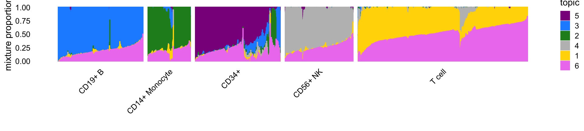
| Version | Author | Date |
|---|---|---|
| 1917832 | Peter Carbonetto | 2021-11-21 |
In particular, topics 1 through 4 closely correspond, respectively, to T cells, CD14+ monocytes (myeloid cells), B cells and natural killer cells. Topic 5 (violet) also closely corresponds to the “CD34+” FACS cell type label but also suggests considerable FACS FACS mislabeling of the CD34+ cells. Topic 6 (magenta) does not correspond to any FACS cell type and as we will it is capturing a different characteristic of the cells—specifically, abundance of ribosomal protein genes. Therefore, we expect the results from the topic-model-based DE analysis for topics 1–4 to most closely resemble the DESeq2 results for the corresponding cell types.
Before entering into this comparison, we first assess accuracy of the MCMC computations in the topic-model-based analysis.
Assessing accuracy of the Monte Carlo estimates
To assess accuracy of the posterior calculations, we perform the DE analysis twice (using different seeds), and compare the posterior mean estimates and z-scores returned by the two de_analysis runs.
load("../output/pbmc-purified/de-pbmc-purified-seed=1.RData")
de1 <- de
load("../output/pbmc-purified/de-pbmc-purified-seed=2.RData")
de2 <- de
rm(de)
The two MCMC estimates of the posterior mean log-fold change (LFC) estimates are largely consistent:
pdat <- data.frame(postmean1 = as.vector(de1$postmean),
                   postmean2 = as.vector(de2$postmean))
ggplot(pdat,aes(x = postmean1,y = postmean2)) +
  geom_point(shape = 21,color = "white",fill = "black",size = 2) +
  geom_abline(intercept = 0,slope = 1,color = "magenta",linetype = "dashed") +
  labs(x = "first posterior mean",y = "second posterior mean") +
  theme_cowplot()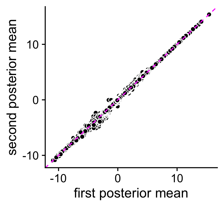
The \(z\)-scores on the other hand are estimated less consistently, presumably because accurately calculating uncertainty in the estimates is harder. Despite this, the \(z\)-scores are still are consistent enough in that it is rare for an LFC to have an lfsr less than 0.05 in one MCMC simulation and not the other (these are the red points in the scatterplot).
pdat <- data.frame(z1 = clamp(as.vector(de1$z),-100,+100),
                   z2 = clamp(as.vector(de2$z),-100,+100),
                   lfsr = factor((de1$lfsr < 0.05) + (de2$lfsr < 0.05)))
ggplot(pdat,aes(x = z1,y = z2,fill = lfsr)) +
  geom_point(shape = 21,color = "white",size = 2) +
  geom_abline(intercept = 0,slope = 1,color = "black",linetype = "dotted") +
  scale_fill_manual(values = c("darkblue","tomato","dodgerblue"),
                    na.value = "white") +
  labs(x = "first z-score",y = "second z-score",fill = "lfsr < 0.05") +
  theme_cowplot()
# Warning: Removed 1546 rows containing missing values (geom_point).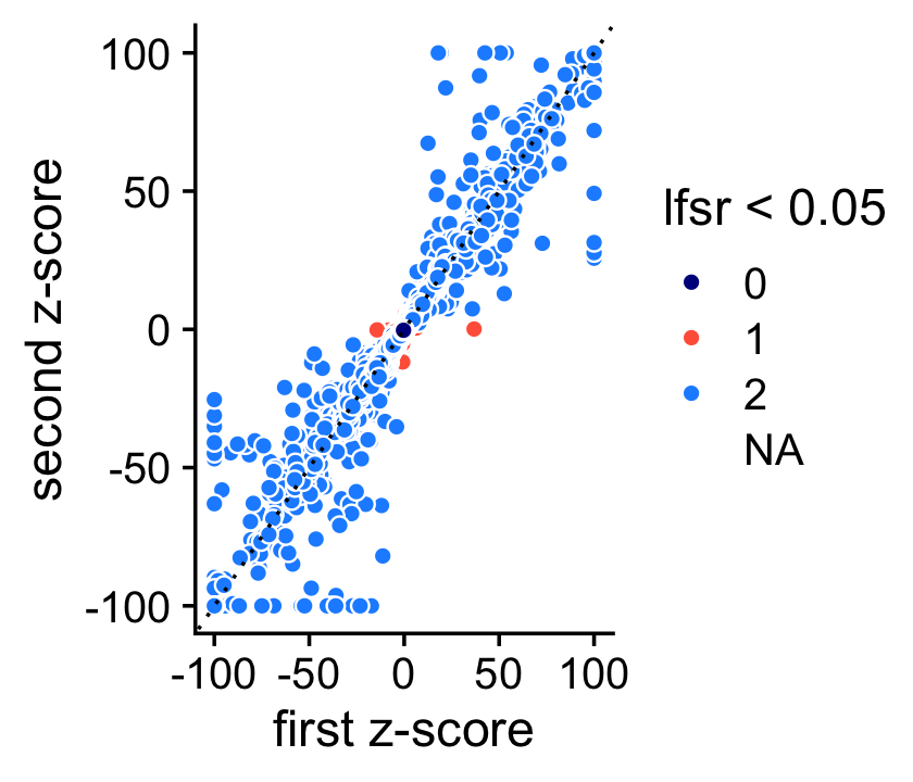
Note: For better visualization \(z\)-scores larger than 100 or smaller than -100 are shown as 100 (or -100).
DESeq2 vs. fastTopics
Next: Compare classical DE analysis (DESeq2) against DE analysis allowing for grades of membership.
sessionInfo()
# R version 3.6.2 (2019-12-12)
# Platform: x86_64-apple-darwin15.6.0 (64-bit)
# Running under: macOS Catalina 10.15.7
#
# Matrix products: default
# BLAS:   /Library/Frameworks/R.framework/Versions/3.6/Resources/lib/libRblas.0.dylib
# LAPACK: /Library/Frameworks/R.framework/Versions/3.6/Resources/lib/libRlapack.dylib
#
# locale:
# [1] en_US.UTF-8/en_US.UTF-8/en_US.UTF-8/C/en_US.UTF-8/en_US.UTF-8
#
# attached base packages:
# [1] stats     graphics  grDevices utils     datasets  methods   base
#
# other attached packages:
# [1] cowplot_1.0.0     ggplot2_3.3.5     fastTopics_0.6-74 Matrix_1.2-18
#
# loaded via a namespace (and not attached):
#  [1] httr_1.4.2         tidyr_1.1.3        jsonlite_1.7.2     viridisLite_0.3.0
#  [5] RcppParallel_4.4.2 assertthat_0.2.1   mixsqp_0.3-46      yaml_2.2.0
#  [9] progress_1.2.2     ggrepel_0.9.1      pillar_1.6.2       backports_1.1.5
# [13] lattice_0.20-38    quantreg_5.54      glue_1.4.2         quadprog_1.5-8
# [17] digest_0.6.23      promises_1.1.0     colorspace_1.4-1   htmltools_0.4.0
# [21] httpuv_1.5.2       pkgconfig_2.0.3    invgamma_1.1       SparseM_1.78
# [25] purrr_0.3.4        scales_1.1.0       whisker_0.4        later_1.0.0
# [29] Rtsne_0.15         MatrixModels_0.4-1 git2r_0.26.1       tibble_3.1.3
# [33] farver_2.0.1       generics_0.0.2     ellipsis_0.3.2     withr_2.4.2
# [37] ashr_2.2-51        pbapply_1.5-1      lazyeval_0.2.2     magrittr_2.0.1
# [41] crayon_1.4.1       mcmc_0.9-6         evaluate_0.14      fs_1.3.1
# [45] fansi_0.4.0        MASS_7.3-51.4      truncnorm_1.0-8    tools_3.6.2
# [49] data.table_1.12.8  prettyunits_1.1.1  hms_1.1.0          lifecycle_1.0.0
# [53] stringr_1.4.0      MCMCpack_1.4-5     plotly_4.9.2       munsell_0.5.0
# [57] irlba_2.3.3        compiler_3.6.2     rlang_0.4.11       grid_3.6.2
# [61] htmlwidgets_1.5.1  labeling_0.3       rmarkdown_2.3      gtable_0.3.0
# [65] DBI_1.1.0          R6_2.4.1           knitr_1.26         dplyr_1.0.7
# [69] utf8_1.1.4         workflowr_1.6.2    rprojroot_1.3-2    stringi_1.4.3
# [73] parallel_3.6.2     SQUAREM_2017.10-1  Rcpp_1.0.7         vctrs_0.3.8
# [77] tidyselect_1.1.1   xfun_0.11          coda_0.19-3