Identify clusters in mixture of FACS-purified PBMC data using topic model
Peter Carbonetto
Last updated: 2020-12-29
Checks: 7 0
Knit directory: single-cell-topics/analysis/
This reproducible R Markdown analysis was created with workflowr (version 1.6.2.9000). The Checks tab describes the reproducibility checks that were applied when the results were created. The Past versions tab lists the development history.
Great! Since the R Markdown file has been committed to the Git repository, you know the exact version of the code that produced these results.
Great job! The global environment was empty. Objects defined in the global environment can affect the analysis in your R Markdown file in unknown ways. For reproduciblity it’s best to always run the code in an empty environment.
The command set.seed(1) was run prior to running the code in the R Markdown file. Setting a seed ensures that any results that rely on randomness, e.g. subsampling or permutations, are reproducible.
Great job! Recording the operating system, R version, and package versions is critical for reproducibility.
Nice! There were no cached chunks for this analysis, so you can be confident that you successfully produced the results during this run.
Great job! Using relative paths to the files within your workflowr project makes it easier to run your code on other machines.
Great! You are using Git for version control. Tracking code development and connecting the code version to the results is critical for reproducibility.
The results in this page were generated with repository version 809d0a1. See the Past versions tab to see a history of the changes made to the R Markdown and HTML files.
Note that you need to be careful to ensure that all relevant files for the analysis have been committed to Git prior to generating the results (you can use wflow_publish or wflow_git_commit). workflowr only checks the R Markdown file, but you know if there are other scripts or data files that it depends on. Below is the status of the Git repository when the results were generated:
Ignored files:
    Ignored:    analysis/figure/
    Ignored:    data/droplet.RData
    Ignored:    data/pbmc_68k.RData
    Ignored:    data/pbmc_purified.RData
    Ignored:    data/pulseseq.RData
    Ignored:    output/droplet/diff-count-droplet.RData
    Ignored:    output/droplet/fits-droplet.RData
    Ignored:    output/droplet/rds/
    Ignored:    output/pbmc-68k/fits-pbmc-68k.RData
    Ignored:    output/pbmc-68k/rds/
    Ignored:    output/pbmc-purified/diff-count-pbmc-purified.RData
    Ignored:    output/pbmc-purified/fits-pbmc-purified.RData
    Ignored:    output/pbmc-purified/rds/
    Ignored:    output/pulseseq/diff-count-pulseseq.RData
    Ignored:    output/pulseseq/fits-pulseseq.RData
    Ignored:    output/pulseseq/rds/

Untracked files:
    Untracked:  analysis/#purified_pbmc_loglik.R#
    Untracked:  analysis/loadings_plot_pbmc_purified.eps
    Untracked:  analysis/pca_cd34_pbmc_purified.png
    Untracked:  analysis/pca_clusters_pbmc_purified.png
    Untracked:  analysis/pca_expression_pbmc_purified.png
    Untracked:  analysis/pca_facs_pbmc_purified.png
    Untracked:  analysis/pca_hexbin_pbmc_purified.eps
    Untracked:  analysis/pca_vs_tsne.eps
    Untracked:  analysis/structure_plot_pbmc_purified.eps
Note that any generated files, e.g. HTML, png, CSS, etc., are not included in this status report because it is ok for generated content to have uncommitted changes.
These are the previous versions of the repository in which changes were made to the R Markdown (analysis/clusters_purified_pbmc.Rmd) and HTML (docs/clusters_purified_pbmc.html) files. If you’ve configured a remote Git repository (see ?wflow_git_remote), click on the hyperlinks in the table below to view the files as they were in that past version.
| File | Version | Author | Date | Message |
|---|---|---|---|---|
| Rmd | 809d0a1 | Peter Carbonetto | 2020-12-29 | workflowr::wflow_publish(“clusters_purified_pbmc.Rmd”, verbose = TRUE) |
| html | 761d2c0 | Peter Carbonetto | 2020-11-29 | Fixed loadings plot in clusters_purified_pbmc analysis. |
| Rmd | 674817c | Peter Carbonetto | 2020-11-29 | workflowr::wflow_publish(“clusters_purified_pbmc.Rmd”) |
| html | aa73ee1 | Peter Carbonetto | 2020-11-29 | Working on adding loadings plot to clusters_purified_pbmc analysis. |
| Rmd | ed4dd7b | Peter Carbonetto | 2020-11-29 | workflowr::wflow_publish(“clusters_purified_pbmc.Rmd”) |
| html | c8fb5be | Peter Carbonetto | 2020-11-29 | Improved PCA expression plots in clusters_purified_pbmc analysis. |
| Rmd | 95f7750 | Peter Carbonetto | 2020-11-29 | workflowr::wflow_publish(“clusters_purified_pbmc.Rmd”) |
| html | a42db50 | Peter Carbonetto | 2020-11-28 | Added PCA expression plots to clusters_purified_pbmc analysis. |
| Rmd | 2de8504 | Peter Carbonetto | 2020-11-28 | workflowr::wflow_publish(“clusters_purified_pbmc.Rmd”) |
| html | 07f6bca | Peter Carbonetto | 2020-11-28 | Made a few minor improvements to the PCA vs. t-SNE + UMAP demo. |
| Rmd | 82b549f | Peter Carbonetto | 2020-11-28 | workflowr::wflow_publish(“clusters_purified_pbmc.Rmd”) |
| html | 3501298 | Peter Carbonetto | 2020-11-28 | Improved Structure plot for purified PBMC data. |
| Rmd | 1f52a7c | Peter Carbonetto | 2020-11-28 | workflowr::wflow_publish(“clusters_purified_pbmc.Rmd”) |
| html | f7e773e | Peter Carbonetto | 2020-11-28 | Build site. |
| Rmd | 31103b8 | Peter Carbonetto | 2020-11-28 | workflowr::wflow_publish(“clusters_purified_pbmc.Rmd”) |
| html | 4781407 | Peter Carbonetto | 2020-11-28 | Made some improvements to the PCA plots in clusters_purified_pbmc. |
| Rmd | 80787eb | Peter Carbonetto | 2020-11-28 | workflowr::wflow_publish(“clusters_purified_pbmc.Rmd”) |
| Rmd | 605ee92 | Peter Carbonetto | 2020-11-28 | Added steps to create PCA plots for paper in clusters_pbmc_purified analysis. |
| Rmd | 39015bd | Peter Carbonetto | 2020-11-28 | Cluster A in PBMC data = dendritic cells. |
| html | 48438b3 | Peter Carbonetto | 2020-11-26 | Added a cluster to the purified PBMC clustering. |
| Rmd | 989e7ac | Peter Carbonetto | 2020-11-26 | workflowr::wflow_publish(“clusters_purified_pbmc.Rmd”) |
| html | c85de93 | Peter Carbonetto | 2020-11-23 | Build site. |
| Rmd | 9389b77 | Peter Carbonetto | 2020-11-23 | workflowr::wflow_publish(“clusters_purified_pbmc.Rmd”) |
| html | e7411a0 | Peter Carbonetto | 2020-11-23 | Added plots comparing PCA with t-SNE and UMAP in |
| Rmd | 9167310 | Peter Carbonetto | 2020-11-23 | workflowr::wflow_publish(“clusters_purified_pbmc.Rmd”) |
| html | 8abec44 | Peter Carbonetto | 2020-11-23 | Added PCA plots to clusters_purified_pbmc analysis. |
| Rmd | a7e6fbc | Peter Carbonetto | 2020-11-23 | Various improvements to the analysis of the PBMC data sets. |
| Rmd | 884b869 | Peter Carbonetto | 2020-11-23 | Working on new plots for clusters_purified_pbmc analysis. |
| Rmd | 4a8b2bd | Peter Carbonetto | 2020-11-23 | A couple additions to clusters_purified_pbmc.Rmd. |
| html | 1845721 | Peter Carbonetto | 2020-11-22 | Added Structure plot to clusters_purified_pbmc. |
| Rmd | 90d201b | Peter Carbonetto | 2020-11-22 | workflowr::wflow_publish(“clusters_purified_pbmc.Rmd”) |
| html | 015e254 | Peter Carbonetto | 2020-11-22 | Fixed up some of the text and plots in clusters_purified_pbmc analysis. |
| Rmd | b512864 | Peter Carbonetto | 2020-11-22 | workflowr::wflow_publish(“clusters_purified_pbmc.Rmd”) |
| html | 7cbd5e9 | Peter Carbonetto | 2020-11-22 | First build of clusters_purified_pbmc page. |
| Rmd | 4e32884 | Peter Carbonetto | 2020-11-22 | workflowr::wflow_publish(“clusters_purified_pbmc.Rmd”) |
Here we perform PCA on the topic proportions to identify clusters in the mixture of FACS-purified PBMC data sets.
Load the packages used in the analysis below, as well as additional functions that we will use to generate some of the plots.
library(Matrix)
library(fastTopics)
library(Rtsne)
library(uwot)
library(ggplot2)
library(cowplot)
source("../code/plots.R")
Load the count data.
load("../data/pbmc_purified.RData")Load the \(K = 6\) Poisson NMF model fit.
fit <- readRDS(file.path("../output/pbmc-purified/rds",
                         "fit-pbmc-purified-scd-ex-k=6.rds"))$fit
fit <- poisson2multinom(fit)
Assess single-cell likelihoods
Identify clusters from principal components
From the PCs of the topic proportions, we define clusters for B-cells, CD14+ cells and CD34+ cells. The remaining cells are assigned to the U cluster (“U” for “unknown”).
pca <- prcomp(fit$L)$x
n   <- nrow(pca)
x   <- rep("U",n)
pc1 <- pca[,1]
pc2 <- pca[,2]
pc3 <- pca[,3]
pc4 <- pca[,4]
pc5 <- pca[,5]
x[pc2 > 0.25] <- "B"
x[pc3 < -0.2 & pc4 < 0.2] <- "CD34+"
x[(pc4 + 0.1)^2 + (pc5 - 0.8)^2 < 0.07] <- "CD14+"
Next, we define clusters for NK cells and dendritic cells from the top 2 PCs of the topic proportions in the U cluster.
rows <- which(x == "U")
n    <- length(rows)
fit2 <- select_loadings(fit,loadings = rows)
pca  <- prcomp(fit2$L)$x
y    <- rep("U",n)
pc1  <- pca[,1]
pc2  <- pca[,2]
pc3  <- pca[,3]
pc4  <- pca[,4]
y[pc1 < -0.3 & 1.1*pc1 < -pc2 - 0.57] <- "NK"
y[pc3 > 0.4 & pc4 < 0.2] <- "dendritic"
x[rows] <- y
Among the remaining cells, we define a cluster for CD8+ cells, noting that this is much less distinct than the other cells. The rest are labeled as T-cells.
rows <- which(x == "U")
n    <- length(rows)
fit2 <- select_loadings(fit,loadings = rows)
pca  <- prcomp(fit2$L)$x
y    <- rep("T",n)
pc1  <- pca[,1]
pc2  <- pca[,2]
y[pc1 < 0.25 & pc2 < -0.15] <- "CD8+"
x[rows] <- y
In summary, we have subdivided the cells into 7 subsets. This plot shows the clustering of the cells projected onto the top two PCs:
cluster_colors <- c("dodgerblue",  # B-cells
                    "forestgreen", # CD14+
                    "darkmagenta", # CD34+
                    "red",         # CD8+
                    "skyblue",     # dendritic
                    "gray",        # NK
                    "darkorange")  # T-cells
samples$cluster <- factor(x)
p1 <- pca_plot(fit,fill = samples$cluster) +
  scale_fill_manual(values = cluster_colors) +
  labs(fill = "cluster")
p2 <- pca_hexbin_plot(fit)
plot_grid(p1,p2,rel_widths = c(10,11))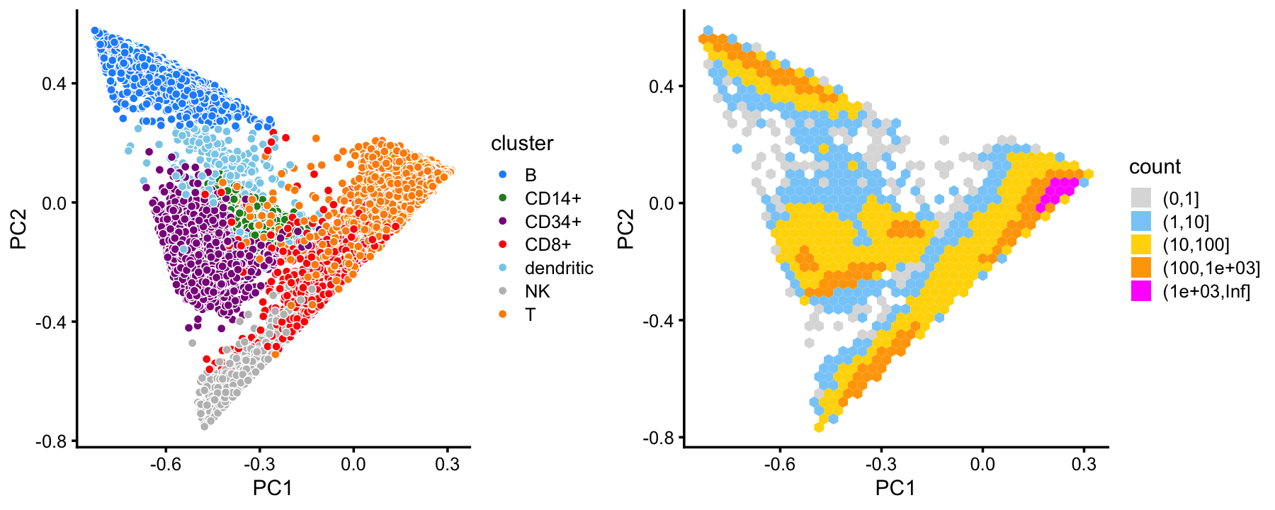
This clustering corresponds well to the Zheng et al (2017) FACS cell populations, although there are some differences.
with(samples,table(celltype,cluster))
#                               cluster
# celltype                           B CD14+ CD34+  CD8+ dendritic    NK     T
#   CD19+ B                      10073     0     0     3         7     0     2
#   CD14+ Monocyte                   8  2420     0     3       156     0    25
#   CD34+                          352   536  8182    20       121     4    17
#   CD4+ T Helper2                   0     0     8    45         9     1 11150
#   CD56+ NK                         0     0    17    82         4  8279     3
#   CD8+ Cytotoxic T                 0     0     0  3146         0    93  6970
#   CD4+/CD45RO+ Memory              0     0    20   355         1     0  9848
#   CD8+/CD45RA+ Naive Cytotoxic     3     0     0    52         2     2 11894
#   CD4+/CD45RA+/CD25- Naive T       1     0     8    27         5     1 10437
#   CD4+/CD25 T Reg                  2     0     2    24         3     0 10232
This good correspondence is also apparent when we layer the FACS cell population labels on the PCA plots:
facs_colors <- c("dodgerblue",  # B-cells
                 "forestgreen", # CD14+
                 "darkmagenta", # CD34+
                 "gray",        # NK cells
                 "tomato",      # cytotoxic T-cells
                 "gold")        # T-cells
x <- as.character(samples$celltype)
x[x == "CD4+ T Helper2" | x == "CD4+/CD45RO+ Memory" |
  x == "CD8+/CD45RA+ Naive Cytotoxic" | x == "CD4+/CD45RA+/CD25- Naive T" |
  x == "CD4+/CD45RA+/CD25- Naive T" | x == "CD4+/CD25 T Reg"] <- "T cell"
x <- factor(x)
p3 <- pca_plot(fit,fill = x) +
  scale_fill_manual(values = facs_colors) +
  labs(fill = "FACS subpopulation")
print(p3)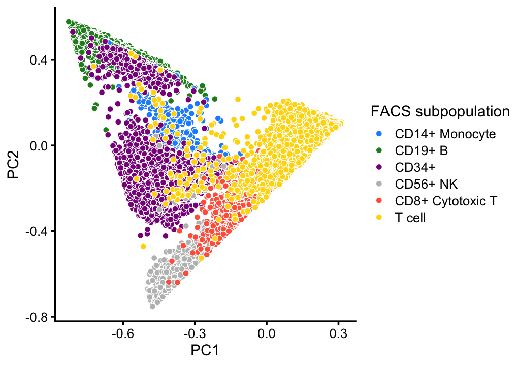
This PCA plot highlights the FACS mis-labeling of the CD34+ cells:
rows <- which(with(samples,
                   cluster == "B" |
                   cluster == "CD14+" |
                   cluster == "CD34+" |
                   cluster == "dendritic"))
p4 <- pca_plot(select_loadings(fit,loadings = rows),
               fill = x[rows,drop = FALSE]) +
  scale_fill_manual(values = facs_colors,drop = FALSE) +
  labs(fill = "FACS subpopulation")
print(p4)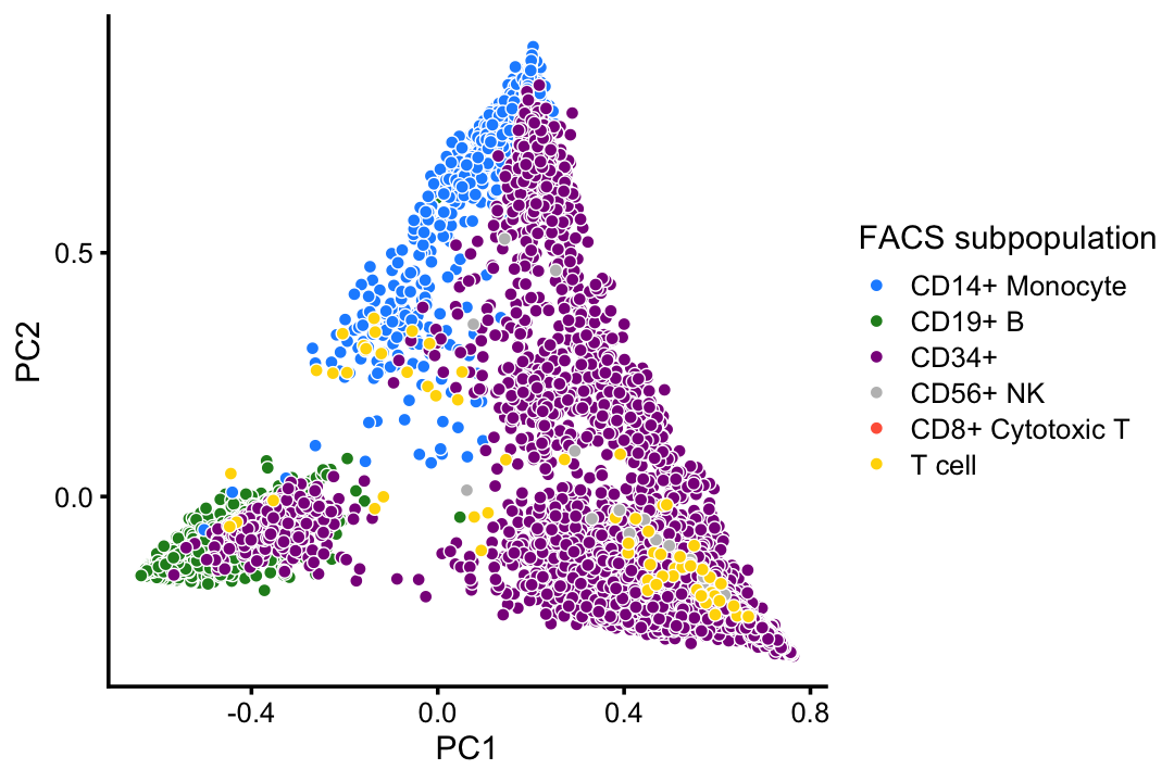
To further drive home this connection, here we layer the PCA plots with expression of cell-type-specific genes, such as CD79A for B-cells:
pca_ggplot_call <- function (dat, pcs, fill.type, fill.label)
  ggplot(dat,aes_string(x = pcs[1],y = pcs[2],color = "y")) +
    geom_point(shape = 20,size = 0.5) +
    labs(x = pcs[1],y = pcs[2],fill = fill.label) +
    scale_color_gradientn(na.value = "skyblue",
                          colors=c("skyblue","gold","darkorange","magenta")) +
    theme_cowplot(font_size = 8) +
    theme(plot.title = element_text(size = 8,face = "plain"))
x   <- counts[,"ENSG00000105369"]
p5a <- pca_plot(select_loadings(fit,loadings = order(x)),
                fill = log10(sort(x)),ggplot_call = pca_ggplot_call) +
       labs(title = "CD79A (B-cells)",color = "log10(count)")
x   <- counts[,"ENSG00000163220"]
p5b <- pca_plot(select_loadings(fit,loadings = order(x)),
                fill = log10(sort(x)),ggplot_call = pca_ggplot_call) +
       labs(title = "S100A9 (CD14+)",color = "log10(count)")
x   <- counts[,"ENSG00000174059"]
p5c <- pca_plot(select_loadings(fit,loadings = order(x)),
                fill = log10(sort(x)),ggplot_call = pca_ggplot_call) +
       labs(title = "CD34 (CD34+)",color = "log10(count)")
x   <- counts[,"ENSG00000197992"]
p5d <- pca_plot(select_loadings(fit,loadings = order(x)),
                fill = log10(sort(x)),ggplot_call = pca_ggplot_call) +
       labs(title = "CLEC9A (dendritic)",color = "log10(count)")
x   <- counts[,"ENSG00000105374"]
p5e <- pca_plot(select_loadings(fit,loadings = order(x)),
                fill = log10(sort(x)),ggplot_call = pca_ggplot_call) +
       labs(title = "NKG7 (NK)",color = "log10(count)")
x    <- counts[,"ENSG00000167286"]
p5f <- pca_plot(select_loadings(fit,loadings = order(x)),
                fill = log10(sort(x)),ggplot_call = pca_ggplot_call) +
       labs(title = "CD3D (T-cells)",color = "log10(count)")
x   <- counts[,"ENSG00000153563"]
p5g <- pca_plot(select_loadings(fit,loadings = order(x)),
                fill = log10(sort(x)),ggplot_call = pca_ggplot_call) +
       labs(title = "CD8A (CD8+ cells)",color = "log10(count)")
plot_grid(p5a,p5b,p5c,
          p5d,p5e,p5f,
          p5g,
          nrow = 3,ncol = 3)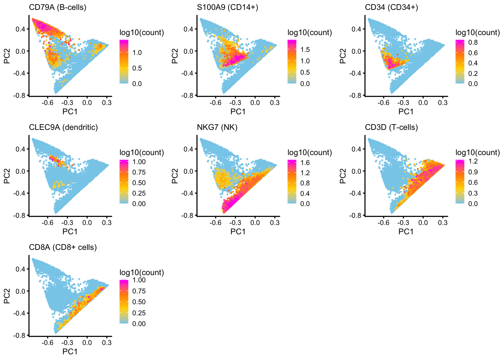
The continuous variation in T-cells captured by topics 1 and 6 suggests CD4+/CD8+ lineage differentiation in T-cells:
x  <- samples$celltype
i  <- names(sort(tapply(fit$L[,1],x,mean)))
x  <- factor(as.character(x),i)
rows <- which(with(samples,!(celltype == "CD19+ B" |
                             celltype == "CD14+ Monocyte" |
                             celltype == "CD34+" |
                             celltype == "CD56+ NK")))
p6 <- loadings_plot(select_loadings(fit,loadings = rows),
                    x = x[rows],k = 1) +
      scale_y_continuous(limits = c(0,1)) +
      labs(y = "topic 1 proportion",title = "")
print(p6)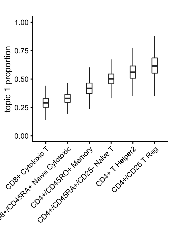
| Version | Author | Date |
|---|---|---|
| 761d2c0 | Peter Carbonetto | 2020-11-29 |
Structure plot
The structure plot summarizes the topic proportions in each of the 7 subsets:
set.seed(1)
topic_colors <- c("gold","forestgreen","dodgerblue","gray",
                  "darkmagenta","violet")
topics <- c(5,3,2,4,1,6)
rows <- sort(c(sample(which(samples$cluster == "B"),1000),
               sample(which(samples$cluster == "CD14+"),300),
               sample(which(samples$cluster == "CD34+"),500),
               sample(which(samples$cluster == "CD8+"),400),
               sample(which(samples$cluster == "NK"),500),
               sample(which(samples$cluster == "T"),1000),
               which(samples$cluster == "dendritic")))
x  <- samples[rows,"cluster"]
x  <- factor(x,c("B","CD14+","CD34+","dendritic","NK","CD8+","T"))
p7 <- structure_plot(select_loadings(fit,loadings = rows),
                     grouping = x,topics = topics,
                     colors = topic_colors[topics],
                     perplexity = c(70,30,30,30,30,30,70),n = Inf,gap = 50,
                     num_threads = 4,verbose = FALSE)
print(p7)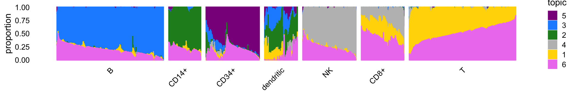
Analysis of single-cell likelihoods
Create scatterplots comparing single-cell likelihoods using a “hard” clustering (based on the FACS subpopulations).
PCA vs. t-SNE and UMAP: an illustration
Here we contrast use of a simple linear dimensionality reduction technique, PCA, with nonlinear dimensionality reduction methods t-SNE and UMAP.
To begin, draw a random subset of 2,000 cells from the B, CD14+ and CD34+ clusters identified above. (The main reason for taking a random subset is that we don’t want to wait a long time for t-SNE and UMAP to complete.)
set.seed(5)
rows <- which(with(samples,
                   cluster == "B" |
                   cluster == "CD14+" |
                   cluster == "CD34+"))
rows <- sort(sample(rows,2000))
fit2 <- select_loadings(fit,loadings = rows)
x    <- samples$cluster[rows,drop = TRUE]
Next, run PCA on the topic proportions for this random subset of 2,000 samples.
p8 <- pca_plot(fit2,fill = x) + labs(fill = "cluster")Run t-SNE on the topic proportions.
tsne <- Rtsne(fit2$L,dims = 2,pca = FALSE,normalize = FALSE,perplexity = 100,
              theta = 0.1,max_iter = 1000,eta = 200,verbose = FALSE)
tsne$x <- tsne$Y
colnames(tsne$x) <- c("tsne1","tsne2")
p9 <- pca_plot(fit2,out.pca = tsne,fill = x) + labs(fill = "cluster")
Then run UMAP on the topic proportions.
out.umap <- umap(fit2$L,n_neighbors = 30,metric = "euclidean",n_epochs = 1000,
                 min_dist = 0.1,scale = "none",learning_rate = 1,
                 verbose = FALSE)
out.umap <- list(x = out.umap)
colnames(out.umap$x) <- c("umap1","umap2")
p10 <- pca_plot(fit2,out.pca = out.umap,fill = x) + labs(fill = "cluster")
Here are the PCA, t-SNE and UMAP 2-d embeddings, side-by-side:
plot_grid(p8,p9,p10,nrow = 1)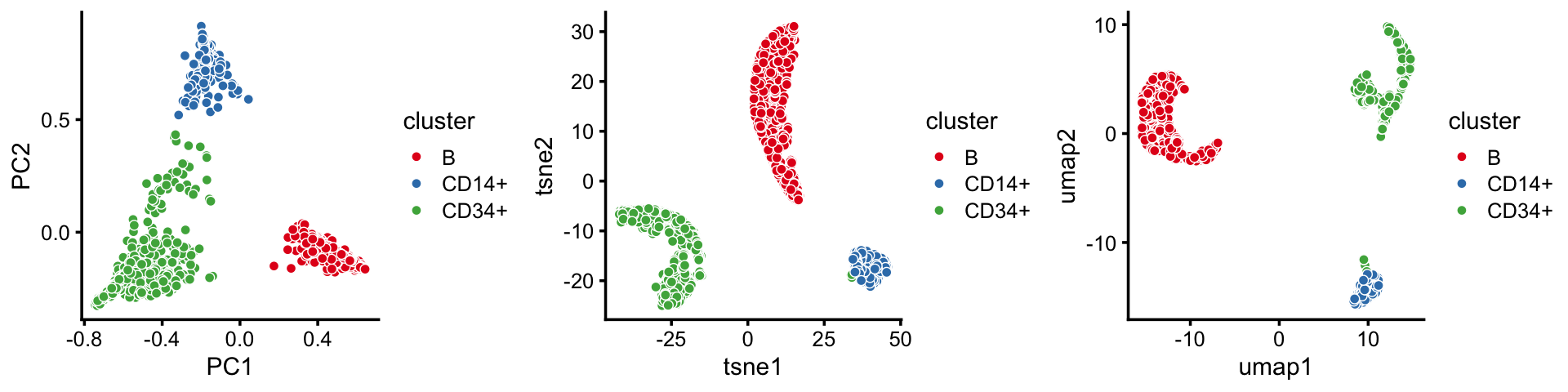
| Version | Author | Date |
|---|---|---|
| e7411a0 | Peter Carbonetto | 2020-11-23 |
By the projection of the samples onto the first two PCs, the B-cells cluster is distinct from the others, whereas the CD14+ and CD34+ cells do not separate as well.
By contrast, this detail is not captured in the t-SNE and UMAP embeddings. This illustrates the tendency of t-SNE and UMAP to accentuate clusters in the data at the risk of distorting or obscuring finer scale substructure.
Note that the first 2 PCs should be sufficient for capturing the full structure in the topic proportions as they explain >96% of the variance:
summary(prcomp(fit2$L))
# Importance of components:
#                           PC1    PC2     PC3     PC4     PC5      PC6
# Standard deviation     0.4831 0.3269 0.10351 0.03397 0.02396 3.49e-16
# Proportion of Variance 0.6618 0.3030 0.03038 0.00327 0.00163 0.00e+00
# Cumulative Proportion  0.6618 0.9647 0.99510 0.99837 1.00000 1.00e+00
Save results
Save the clustering of the PBMC data to an RDS file.
saveRDS(samples,"clustering-pbmc-purified.rds")
sessionInfo()
# R version 3.6.2 (2019-12-12)
# Platform: x86_64-apple-darwin15.6.0 (64-bit)
# Running under: macOS Catalina 10.15.7
#
# Matrix products: default
# BLAS:   /Library/Frameworks/R.framework/Versions/3.6/Resources/lib/libRblas.0.dylib
# LAPACK: /Library/Frameworks/R.framework/Versions/3.6/Resources/lib/libRlapack.dylib
#
# locale:
# [1] en_US.UTF-8/en_US.UTF-8/en_US.UTF-8/C/en_US.UTF-8/en_US.UTF-8
#
# attached base packages:
# [1] stats     graphics  grDevices utils     datasets  methods   base
#
# other attached packages:
# [1] cowplot_1.0.0     ggplot2_3.3.0     uwot_0.1.8        Rtsne_0.15
# [5] fastTopics_0.4-11 Matrix_1.2-18
#
# loaded via a namespace (and not attached):
#  [1] ggrepel_0.9.0        Rcpp_1.0.5           lattice_0.20-38
#  [4] FNN_1.1.3            tidyr_1.0.0          prettyunits_1.1.1
#  [7] assertthat_0.2.1     zeallot_0.1.0        rprojroot_1.3-2
# [10] digest_0.6.23        R6_2.4.1             backports_1.1.5
# [13] MatrixModels_0.4-1   evaluate_0.14        coda_0.19-3
# [16] httr_1.4.2           pillar_1.4.3         rlang_0.4.5
# [19] progress_1.2.2       lazyeval_0.2.2       data.table_1.12.8
# [22] irlba_2.3.3          SparseM_1.78         hexbin_1.28.0
# [25] whisker_0.4          rmarkdown_2.3        labeling_0.3
# [28] stringr_1.4.0        htmlwidgets_1.5.1    munsell_0.5.0
# [31] compiler_3.6.2       httpuv_1.5.2         xfun_0.11
# [34] pkgconfig_2.0.3      mcmc_0.9-6           htmltools_0.4.0
# [37] tidyselect_0.2.5     tibble_2.1.3         workflowr_1.6.2.9000
# [40] quadprog_1.5-8       viridisLite_0.3.0    crayon_1.3.4
# [43] dplyr_0.8.3          withr_2.1.2          later_1.0.0
# [46] MASS_7.3-51.4        grid_3.6.2           jsonlite_1.6
# [49] gtable_0.3.0         lifecycle_0.1.0      git2r_0.26.1
# [52] magrittr_1.5         scales_1.1.0         RcppParallel_4.4.2
# [55] stringi_1.4.3        farver_2.0.1         fs_1.3.1
# [58] promises_1.1.0       vctrs_0.2.1          tools_3.6.2
# [61] glue_1.3.1           purrr_0.3.3          hms_0.5.2
# [64] yaml_2.2.0           colorspace_1.4-1     plotly_4.9.2
# [67] knitr_1.26           quantreg_5.54        MCMCpack_1.4-5