Assess Poisson NMF fits in droplet data
Peter Carbonetto
Last updated: 2020-08-09
Checks: 7 0
Knit directory: single-cell-topics/analysis/
This reproducible R Markdown analysis was created with workflowr (version 1.6.2.9000). The Checks tab describes the reproducibility checks that were applied when the results were created. The Past versions tab lists the development history.
Great! Since the R Markdown file has been committed to the Git repository, you know the exact version of the code that produced these results.
Great job! The global environment was empty. Objects defined in the global environment can affect the analysis in your R Markdown file in unknown ways. For reproduciblity it’s best to always run the code in an empty environment.
The command set.seed(1) was run prior to running the code in the R Markdown file. Setting a seed ensures that any results that rely on randomness, e.g. subsampling or permutations, are reproducible.
Great job! Recording the operating system, R version, and package versions is critical for reproducibility.
Nice! There were no cached chunks for this analysis, so you can be confident that you successfully produced the results during this run.
Great job! Using relative paths to the files within your workflowr project makes it easier to run your code on other machines.
Great! You are using Git for version control. Tracking code development and connecting the code version to the results is critical for reproducibility.
The results in this page were generated with repository version 1ef2ac6. See the Past versions tab to see a history of the changes made to the R Markdown and HTML files.
Note that you need to be careful to ensure that all relevant files for the analysis have been committed to Git prior to generating the results (you can use wflow_publish or wflow_git_commit). workflowr only checks the R Markdown file, but you know if there are other scripts or data files that it depends on. Below is the status of the Git repository when the results were generated:
Ignored files:
    Ignored:    output/droplet/fits-droplet.RData
Note that any generated files, e.g. HTML, png, CSS, etc., are not included in this status report because it is ok for generated content to have uncommitted changes.
These are the previous versions of the repository in which changes were made to the R Markdown (analysis/assess_fits_droplet.Rmd) and HTML (docs/assess_fits_droplet.html) files. If you’ve configured a remote Git repository (see ?wflow_git_remote), click on the hyperlinks in the table below to view the files as they were in that past version.
| File | Version | Author | Date | Message |
|---|---|---|---|---|
| Rmd | 1ef2ac6 | Peter Carbonetto | 2020-08-09 | wflow_publish(“assess_fits_droplet.Rmd”) |
| Rmd | 68d8a4a | Peter Carbonetto | 2020-08-09 | Added comments and made minor adjustments to create_progress_plots. |
| Rmd | 94c632a | Peter Carbonetto | 2020-08-09 | Working on assess_fits_droplet analysis. |
Here we compare the quality of the fits obtained from the different updates (EM, CCD, SCD, with and without extrapolation), and with different \(k\).
These are the packages used in the analysis below.
library(fastTopics)
library(ggplot2)
library(cowplot)
source("../code/functions_for_assessing_fits.R")
Load the results of running fit_poisson_nmf on the purified PBMC data, with different algorithms, and for various choices of \(k\) (the number of “topics”). These results were then compiled into a single file using the compile_poisson_nmf_fits.R script.
load("../output/droplet/fits-droplet.RData")This plot shows the improvement in the log-likelihood as the rank, \(k\), is increased. The log-likelihoods are shown relative to the log-likelihood at rank \(k = 2\).
plot_loglik_vs_rank(fits)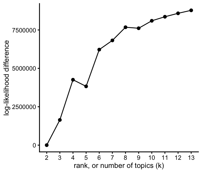
As expected, the likelihood improves with larger rank, \(k\), although these improvements are large for smaller \(k\), and more gradual as \(k\) gets larger.
This first set of plots shows the improvement in the fit over time, for all choices of \(k\), and for each of the three optimization methods (EM, CCD, SCD), with and without the extrapolation scheme. The quality of the fit is measured by the log-likelihood, relative to the best log-likelihood that was identified among all methods compared.
create_progress_plots(dat,fits,"loglik")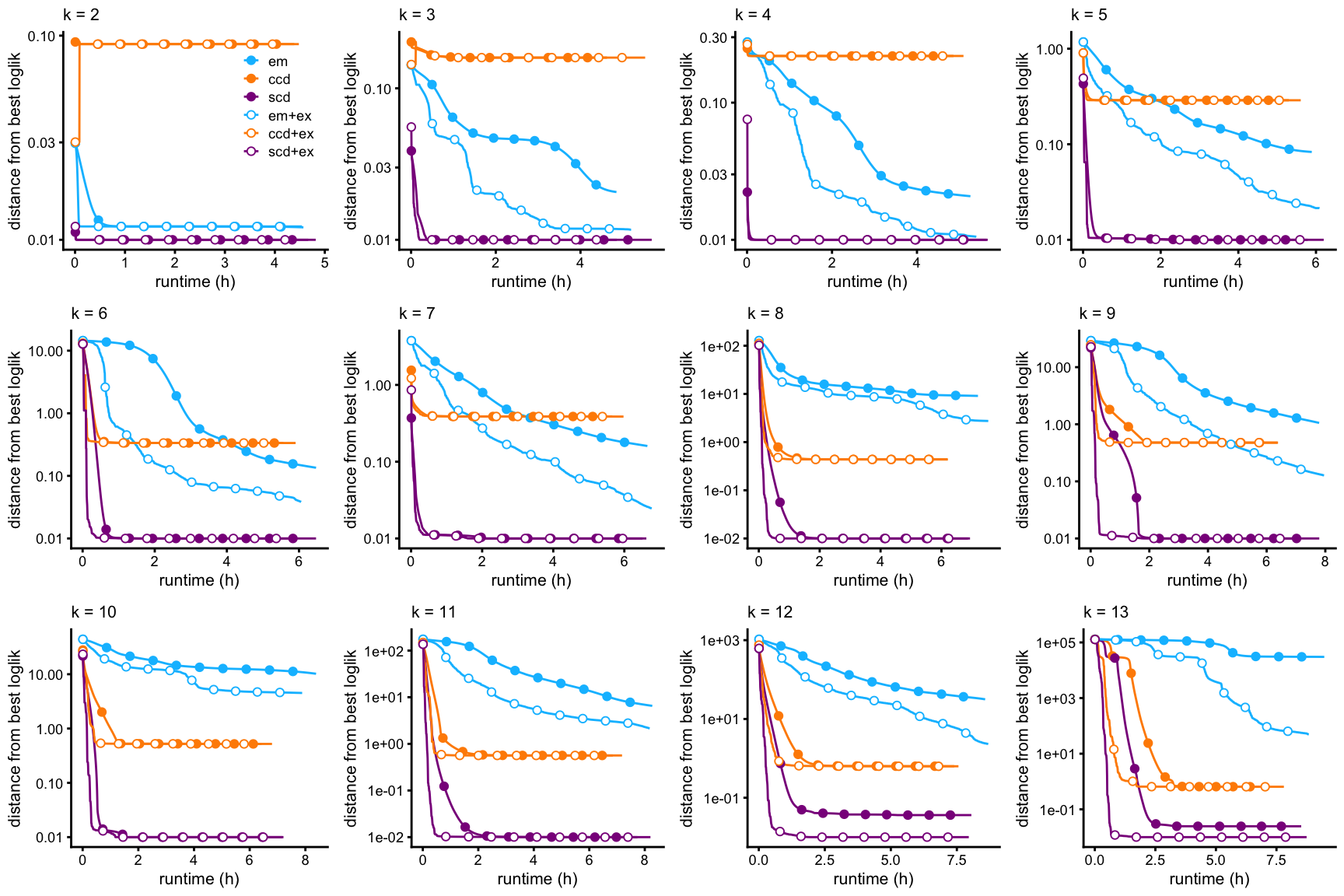
The second set of plots shows the evolution of Karush-Kuhn-Tucker (KKT) residuals over time; the KKT residuals should vanish near a stationary point of the log-likelihood, so looking at the largest KKT residual can be used to assess how close we are to a solution.
Note that, unlike the likelihood, the residuals of the KKT conditions are not expected to decrease monotonically over time.
create_progress_plots(dat,fits,"res")
A few striking trends emerge from these plots:
EM (with or without extrapolation) almost always provides the worst fit, and progresses very slowly to a solution.
CCD (with or without extrapolation) usually, but not always, progresses to a solution much more quickly than EM, and identifies a better MLE.
SCD (with or without extrapolation) almost always progresses more rapidly to a solution.
SCD with extrapolation always progresses more rapidly to a solution, and always identifies the best local solution.
sessionInfo()
# R version 3.6.2 (2019-12-12)
# Platform: x86_64-apple-darwin15.6.0 (64-bit)
# Running under: macOS Catalina 10.15.5
#
# Matrix products: default
# BLAS:   /Library/Frameworks/R.framework/Versions/3.6/Resources/lib/libRblas.0.dylib
# LAPACK: /Library/Frameworks/R.framework/Versions/3.6/Resources/lib/libRlapack.dylib
#
# locale:
# [1] en_US.UTF-8/en_US.UTF-8/en_US.UTF-8/C/en_US.UTF-8/en_US.UTF-8
#
# attached base packages:
# [1] stats     graphics  grDevices utils     datasets  methods   base
#
# other attached packages:
# [1] cowplot_1.0.0      ggplot2_3.3.0      fastTopics_0.3-145
#
# loaded via a namespace (and not attached):
#  [1] ggrepel_0.9.0        Rcpp_1.0.3           lattice_0.20-38
#  [4] tidyr_1.0.0          prettyunits_1.1.1    assertthat_0.2.1
#  [7] zeallot_0.1.0        rprojroot_1.3-2      digest_0.6.23
# [10] R6_2.4.1             backports_1.1.5      MatrixModels_0.4-1
# [13] evaluate_0.14        coda_0.19-3          httr_1.4.1
# [16] pillar_1.4.3         rlang_0.4.5          progress_1.2.2
# [19] lazyeval_0.2.2       data.table_1.12.8    irlba_2.3.3
# [22] SparseM_1.78         whisker_0.4          Matrix_1.2-18
# [25] rmarkdown_2.3        labeling_0.3         Rtsne_0.15
# [28] stringr_1.4.0        htmlwidgets_1.5.1    munsell_0.5.0
# [31] compiler_3.6.2       httpuv_1.5.2         xfun_0.11
# [34] pkgconfig_2.0.3      mcmc_0.9-6           htmltools_0.4.0
# [37] tidyselect_0.2.5     tibble_2.1.3         workflowr_1.6.2.9000
# [40] quadprog_1.5-8       viridisLite_0.3.0    crayon_1.3.4
# [43] dplyr_0.8.3          withr_2.1.2          later_1.0.0
# [46] MASS_7.3-51.4        grid_3.6.2           jsonlite_1.6
# [49] gtable_0.3.0         lifecycle_0.1.0      git2r_0.26.1
# [52] magrittr_1.5         scales_1.1.0         RcppParallel_4.4.4
# [55] stringi_1.4.3        farver_2.0.1         fs_1.3.1
# [58] promises_1.1.0       vctrs_0.2.1          tools_3.6.2
# [61] glue_1.3.1           purrr_0.3.3          hms_0.5.2
# [64] yaml_2.2.0           colorspace_1.4-1     plotly_4.9.2
# [67] knitr_1.26           quantreg_5.54        MCMCpack_1.4-5