DE analysis using a topic model: evaluation using simulated data
Peter Carbonetto
Last updated: 2021-10-11
Checks: 7 0
Knit directory: single-cell-topics/analysis/
This reproducible R Markdown analysis was created with workflowr (version 1.6.2). The Checks tab describes the reproducibility checks that were applied when the results were created. The Past versions tab lists the development history.
Great! Since the R Markdown file has been committed to the Git repository, you know the exact version of the code that produced these results.
Great job! The global environment was empty. Objects defined in the global environment can affect the analysis in your R Markdown file in unknown ways. For reproduciblity it’s best to always run the code in an empty environment.
The command set.seed(1) was run prior to running the code in the R Markdown file. Setting a seed ensures that any results that rely on randomness, e.g. subsampling or permutations, are reproducible.
Great job! Recording the operating system, R version, and package versions is critical for reproducibility.
Nice! There were no cached chunks for this analysis, so you can be confident that you successfully produced the results during this run.
Great job! Using relative paths to the files within your workflowr project makes it easier to run your code on other machines.
Great! You are using Git for version control. Tracking code development and connecting the code version to the results is critical for reproducibility.
The results in this page were generated with repository version e2577f1. See the Past versions tab to see a history of the changes made to the R Markdown and HTML files.
Note that you need to be careful to ensure that all relevant files for the analysis have been committed to Git prior to generating the results (you can use wflow_publish or wflow_git_commit). workflowr only checks the R Markdown file, but you know if there are other scripts or data files that it depends on. Below is the status of the Git repository when the results were generated:
Ignored files:
    Ignored:    data/droplet.RData
    Ignored:    data/pbmc_68k.RData
    Ignored:    data/pbmc_purified.RData
    Ignored:    data/pulseseq.RData
    Ignored:    output/droplet/diff-count-droplet.RData
    Ignored:    output/droplet/fits-droplet.RData
    Ignored:    output/droplet/rds/
    Ignored:    output/pbmc-68k/fits-pbmc-68k.RData
    Ignored:    output/pbmc-68k/rds/
    Ignored:    output/pbmc-purified/fits-pbmc-purified.RData
    Ignored:    output/pbmc-purified/rds/
    Ignored:    output/pulseseq/diff-count-pulseseq.RData
    Ignored:    output/pulseseq/fits-pulseseq.RData
    Ignored:    output/pulseseq/rds/

Untracked files:
    Untracked:  plots/
Note that any generated files, e.g. HTML, png, CSS, etc., are not included in this status report because it is ok for generated content to have uncommitted changes.
These are the previous versions of the repository in which changes were made to the R Markdown (analysis/de_analysis_detailed_look.Rmd) and HTML (docs/de_analysis_detailed_look.html) files. If you’ve configured a remote Git repository (see ?wflow_git_remote), click on the hyperlinks in the table below to view the files as they were in that past version.
| File | Version | Author | Date | Message |
|---|---|---|---|---|
| Rmd | e2577f1 | Peter Carbonetto | 2021-10-11 | Working on the data simulation step in the de_analysis_detailed_look |
| html | cd17ccf | Peter Carbonetto | 2021-10-09 | Initial build of the de_analysis_detailed_look workflowr page. |
| Rmd | b8e1fe8 | Peter Carbonetto | 2021-10-09 | workflowr::wflow_publish(“de_analysis_detailed_look.Rmd”) |
| Rmd | 888ea7d | Peter Carbonetto | 2021-10-08 | I have an initial implementation of function simulate_twotopic_scrnaseq_data used to evaluate the de_analysis methods in fastTopics. |
Add summary of the analysis here.
Load the packages used in the analysis below, and some additional functions for simulating the data.
library(Matrix)
library(fastTopics)
library(MCMCpack)
library(ggplot2)
library(cowplot)
source("../code/de_eval_functions.R")
Simulate UMI counts
We begin by simulating counts intended to “mimic” UMI count data from a single-cell RNA sequencing experiment. In particular, we simulate counts \(x_{ij}\) from a Poisson NMF model \(x_{ij} \sim \mathrm{Poisson}(\lambda_{ij})\), such that \(\lambda_{ij} = \sum_{k=1}^K l_{ik} f_{jk}\). For now we focus our attention on the case of \(K = 2\) topics (e.g., two cell types or two cell states) to simplify the analysis; comparing gene expression between three or topics brings some additional complications which aren’t necessary for vunderstanding the properties of the new DE methods.
set.seed(1)
dat <- simulate_twotopic_umi_data()
X <- dat$X
The multinomial sample sizes (the total count in each cell) were simulated to be normally distributed on the (base-10) log scale with mean 3.2 and s.d. 0.2:
s <- rowSums(X)
ggplot(data.frame(s = log10(s)),aes(x = s)) +
  geom_histogram(color = "white",fill = "black",bins = 32) +
  labs(x = "log10 size",y = "cells") +
  theme_cowplot()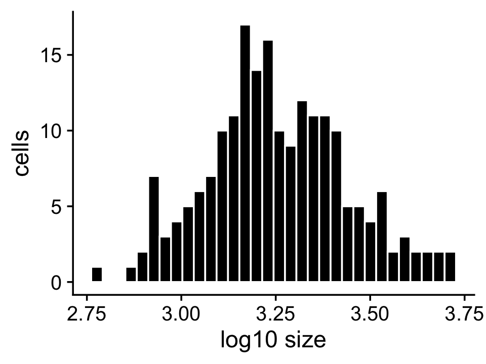
mean(log10(s))
sd(log10(s))
# [1] 3.25348
# [1] 0.1849638
We have simulated the expression rates so that they are normally distributed on the log scale:
ggplot(data.frame(f = as.vector(dat$F)),aes(x = log10(f))) +
  geom_histogram(color = "white",fill = "black",bins = 32) +
  labs(x = "log10 expression rate",y = "genes") +
  theme_cowplot()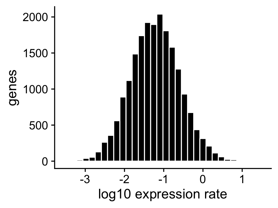
The log-fold changes (LFCs) in expression are simulated to be roughly t-distibuted with 1.7 degrees of freedom, \(\mathrm{lfc\)} 0.7t_{1.7}$:
lfc <- log2(dat$F[,1]/dat$F[,2])
mean(lfc == 0)
ggplot(data.frame(lfc = lfc[lfc != 0]),aes(x = lfc)) +
geom_histogram(color = "white",fill = "black",bins = 32) +
  theme_cowplot()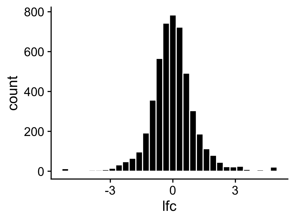
# [1] 0.5002
sessionInfo()
# R version 3.6.2 (2019-12-12)
# Platform: x86_64-apple-darwin15.6.0 (64-bit)
# Running under: macOS Catalina 10.15.7
#
# Matrix products: default
# BLAS:   /Library/Frameworks/R.framework/Versions/3.6/Resources/lib/libRblas.0.dylib
# LAPACK: /Library/Frameworks/R.framework/Versions/3.6/Resources/lib/libRlapack.dylib
#
# locale:
# [1] en_US.UTF-8/en_US.UTF-8/en_US.UTF-8/C/en_US.UTF-8/en_US.UTF-8
#
# attached base packages:
# [1] stats     graphics  grDevices utils     datasets  methods   base
#
# other attached packages:
# [1] cowplot_1.0.0     ggplot2_3.3.5     MCMCpack_1.4-5    MASS_7.3-51.4
# [5] coda_0.19-3       fastTopics_0.6-70 Matrix_1.2-18
#
# loaded via a namespace (and not attached):
#  [1] httr_1.4.2         tidyr_1.1.3        jsonlite_1.7.2     viridisLite_0.3.0
#  [5] RcppParallel_4.4.2 assertthat_0.2.1   mixsqp_0.3-46      yaml_2.2.0
#  [9] progress_1.2.2     ggrepel_0.9.1      pillar_1.6.2       backports_1.1.5
# [13] lattice_0.20-38    quantreg_5.54      glue_1.4.2         quadprog_1.5-8
# [17] digest_0.6.23      promises_1.1.0     colorspace_1.4-1   htmltools_0.4.0
# [21] httpuv_1.5.2       pkgconfig_2.0.3    invgamma_1.1       SparseM_1.78
# [25] purrr_0.3.4        scales_1.1.0       whisker_0.4        later_1.0.0
# [29] Rtsne_0.15         MatrixModels_0.4-1 git2r_0.26.1       tibble_3.1.3
# [33] farver_2.0.1       generics_0.0.2     ellipsis_0.3.2     withr_2.4.2
# [37] ashr_2.2-51        lazyeval_0.2.2     magrittr_2.0.1     crayon_1.4.1
# [41] mcmc_0.9-6         evaluate_0.14      fs_1.3.1           fansi_0.4.0
# [45] truncnorm_1.0-8    tools_3.6.2        data.table_1.12.8  prettyunits_1.1.1
# [49] hms_1.1.0          lifecycle_1.0.0    stringr_1.4.0      plotly_4.9.2
# [53] munsell_0.5.0      irlba_2.3.3        compiler_3.6.2     rlang_0.4.11
# [57] grid_3.6.2         htmlwidgets_1.5.1  labeling_0.3       rmarkdown_2.3
# [61] gtable_0.3.0       DBI_1.1.0          R6_2.4.1           knitr_1.26
# [65] dplyr_1.0.7        utf8_1.1.4         workflowr_1.6.2    rprojroot_1.3-2
# [69] stringi_1.4.3      parallel_3.6.2     SQUAREM_2017.10-1  Rcpp_1.0.7
# [73] vctrs_0.3.8        tidyselect_1.1.1   xfun_0.11