Motorcycle Acceleration example
Zhengrong Xing, Peter Carbonetto and Matthew Stephens
Last updated: 2018-12-07
workflowr checks: (Click a bullet for more information)-
✔ R Markdown file: up-to-date
Great! Since the R Markdown file has been committed to the Git repository, you know the exact version of the code that produced these results.
-
✔ Environment: empty
Great job! The global environment was empty. Objects defined in the global environment can affect the analysis in your R Markdown file in unknown ways. For reproduciblity it’s best to always run the code in an empty environment.
-
✔ Seed:
set.seed(1)The command
set.seed(1)was run prior to running the code in the R Markdown file. Setting a seed ensures that any results that rely on randomness, e.g. subsampling or permutations, are reproducible. -
✔ Session information: recorded
Great job! Recording the operating system, R version, and package versions is critical for reproducibility.
-
Great! You are using Git for version control. Tracking code development and connecting the code version to the results is critical for reproducibility. The version displayed above was the version of the Git repository at the time these results were generated.✔ Repository version: 5c617d0
Note that you need to be careful to ensure that all relevant files for the analysis have been committed to Git prior to generating the results (you can usewflow_publishorwflow_git_commit). workflowr only checks the R Markdown file, but you know if there are other scripts or data files that it depends on. Below is the status of the Git repository when the results were generated:
Note that any generated files, e.g. HTML, png, CSS, etc., are not included in this status report because it is ok for generated content to have uncommitted changes.Ignored files: Ignored: dsc/code/Wavelab850/MEXSource/CPAnalysis.mexmac Ignored: dsc/code/Wavelab850/MEXSource/DownDyadHi.mexmac Ignored: dsc/code/Wavelab850/MEXSource/DownDyadLo.mexmac Ignored: dsc/code/Wavelab850/MEXSource/FAIPT.mexmac Ignored: dsc/code/Wavelab850/MEXSource/FCPSynthesis.mexmac Ignored: dsc/code/Wavelab850/MEXSource/FMIPT.mexmac Ignored: dsc/code/Wavelab850/MEXSource/FWPSynthesis.mexmac Ignored: dsc/code/Wavelab850/MEXSource/FWT2_PO.mexmac Ignored: dsc/code/Wavelab850/MEXSource/FWT_PBS.mexmac Ignored: dsc/code/Wavelab850/MEXSource/FWT_PO.mexmac Ignored: dsc/code/Wavelab850/MEXSource/FWT_TI.mexmac Ignored: dsc/code/Wavelab850/MEXSource/IAIPT.mexmac Ignored: dsc/code/Wavelab850/MEXSource/IMIPT.mexmac Ignored: dsc/code/Wavelab850/MEXSource/IWT2_PO.mexmac Ignored: dsc/code/Wavelab850/MEXSource/IWT_PBS.mexmac Ignored: dsc/code/Wavelab850/MEXSource/IWT_PO.mexmac Ignored: dsc/code/Wavelab850/MEXSource/IWT_TI.mexmac Ignored: dsc/code/Wavelab850/MEXSource/LMIRefineSeq.mexmac Ignored: dsc/code/Wavelab850/MEXSource/MedRefineSeq.mexmac Ignored: dsc/code/Wavelab850/MEXSource/UpDyadHi.mexmac Ignored: dsc/code/Wavelab850/MEXSource/UpDyadLo.mexmac Ignored: dsc/code/Wavelab850/MEXSource/WPAnalysis.mexmac Ignored: dsc/code/Wavelab850/MEXSource/dct_ii.mexmac Ignored: dsc/code/Wavelab850/MEXSource/dct_iii.mexmac Ignored: dsc/code/Wavelab850/MEXSource/dct_iv.mexmac Ignored: dsc/code/Wavelab850/MEXSource/dst_ii.mexmac Ignored: dsc/code/Wavelab850/MEXSource/dst_iii.mexmac Untracked files: Untracked: analysis/gauss_dsc.Rmd
Expand here to see past versions:
| File | Version | Author | Date | Message |
|---|---|---|---|---|
| Rmd | a09d13e | Peter Carbonetto | 2018-11-09 | Adjusted setup steps in a few of the R Markdown files. |
| Rmd | f9f193c | Peter Carbonetto | 2018-11-07 | Revised setup instructions for a couple .Rmd files. |
| Rmd | 3b7071b | Peter Carbonetto | 2018-11-06 | wflow_publish(“motorcycle.Rmd”) |
| html | 3ce045f | Peter Carbonetto | 2018-11-06 | Added explanatory text to motorcycle example. |
| Rmd | 4a73ed9 | Peter Carbonetto | 2018-11-06 | wflow_publish(“motorcycle.Rmd”) |
| Rmd | fd51be8 | Peter Carbonetto | 2018-11-06 | wflow_publish(“motorcycle.Rmd”) |
| html | fdc9c33 | Peter Carbonetto | 2018-11-06 | Build site. |
| Rmd | 1ab1447 | Peter Carbonetto | 2018-11-06 | wflow_publish(“motorcycle.Rmd”) |
| Rmd | f0059b3 | Peter Carbonetto | 2018-11-06 | wflow_publish(“motorcycle.Rmd”) |
| Rmd | 507a261 | Peter Carbonetto | 2018-11-06 | Having trouble re-building spikesdemo.html. |
| Rmd | 7f2ef79 | Peter Carbonetto | 2018-10-10 | wflow_publish(“motorcycle.Rmd”) |
| Rmd | 3b3d373 | Peter Carbonetto | 2018-10-09 | Some more improvements to the motorcycle example. |
| Rmd | 757462c | Peter Carbonetto | 2018-10-09 | Working on motorcycle .Rmd example. |
This is an illustration of “smoothing via adaptive shrinkage” (SMASH) applied to the Motorcycle Accident data. This implements the “illustrative application” presented in Sec. 5.1 of the manuscript.
Initial setup instructions
To run this example on your own computer, please follow these setup instructions. These instructions assume you already have R and/or RStudio installed on your computer.
Download or clone the git repository on your computer.
Launch R, and change the working directory to be the “analysis” folder inside your local copy of the git repository.
Install the devtools, wavethresh and EbayesThresh packages used here and in the code below:
install.packages(c("devtools","wavethresh","EbayesThresh"))Finally, install the smashr package from GitHub:
devtools::install_github("stephenslab/smashr")See the “Session Info” at the bottom for the versions of the software and R packages that were used to generate the results shown below.
Set up R environment
Load the MASS, lattice wavethresh, EbayesThresh and smashr packages. The MASS package is loaded only for the Motorcycle Accident data. Some additional functions are defined in functions.motorcycle.R.
library(MASS)
library(lattice)
library(smashr)
library(wavethresh)
library(EbayesThresh)
source("../code/motorcycle.functions.R")
Note that the MASS and lattice packages are included in most standard R installations, so you probably don’t need to install these packages separately.
Prepare data for SMASH
Load the motorcycle data from the MASS package, and order the data points by time.
data(mcycle)
x.ini.mc <- sort(mcycle$times)
y.ini.mc <- mcycle$accel[order(mcycle$times)]
Run SMASH
Apply SMASH to the Motorcycle Accident data set.
res.mc <- smash.wrapper(x.ini.mc,y.ini.mc)Summarize results of SMASH analysis
Create a plot showing the Motorcycle Accident data and the smash estimates (with the dashed red lines showing the confidence intervals).
plot(res.mc$x,res.mc$mu.est,type = "l",
     ylim = c(min(res.mc$y - 2 * sqrt(res.mc$var.est)),
              max(res.mc$y + 2 * sqrt(res.mc$var.est))),
     xlab = "time (ms)", ylab = "acceleration (g)",lwd = 2,
     col = "darkorange",xlim = c(0,60),xaxp = c(0,60,6))
lines(res.mc$x, res.mc$mu.est + 2*sqrt(res.mc$var.est),lty = 5,
     lwd = 2,col = "dodgerblue")
lines(res.mc$x,res.mc$mu.est - 2*sqrt(res.mc$var.est),
      lty = 5,lwd = 2,col = "dodgerblue")
points(res.mc$x,res.mc$y,pch = 1,cex = 1,col = "black")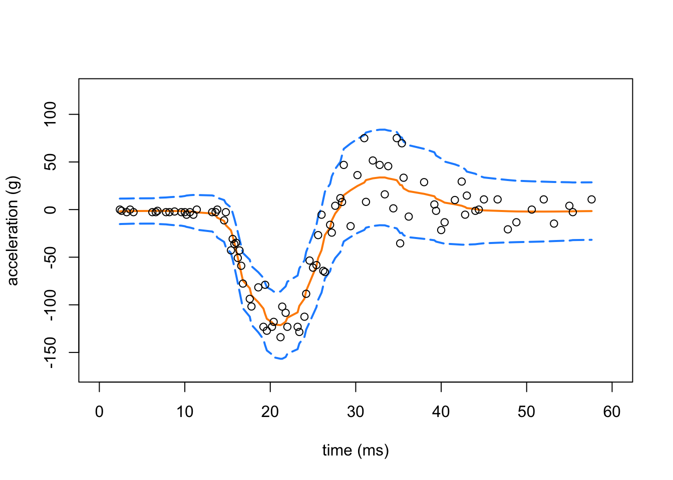
Apply SMASH again, this time assuming equal variances
Apply SMASH (assuming equal variances) to the Motorcycle Accident data set.
res.cons.mc <- smash.cons.wrapper(x.ini.mc,y.ini.mc)Apply TI thresholding to the Motorcycle Accident data
Apply TI thresholding to the Motorcycle Accident data set.
res.ti.cons.mc <- tithresh.cons.wrapper(x.ini.mc,y.ini.mc)Apply TI thresholding to the Motorcycle Accident data, this time using the variances estimated by SMASH.
res.ti.mc <- tithresh.wrapper(x.ini.mc,y.ini.mc)Compare results from all methods
In this second plot, we compare the mean estimate provided by SMASH (with heteroskedastic variances; orange line) against homoskedastic SMASH (dotted, light blue line).
plot(res.mc$x,res.mc$mu.est,type = "l",
     ylim = c(min(res.mc$y - 2 * sqrt(res.mc$var.est)),
              max(res.mc$y + 2 * sqrt(res.mc$var.est))),
     xlab = "time (ms)",ylab = "acceleration (g)",lwd = 2,
     col = "darkorange",xlim = c(0,60),xaxp = c(0,60,6))
lines(res.cons.mc$x,res.cons.mc$mu.est,lwd = 2,lty = "dotted",
      col = "dodgerblue")
points(res.mc$x,res.mc$y,pch = 1,cex = 0.8,col = "black")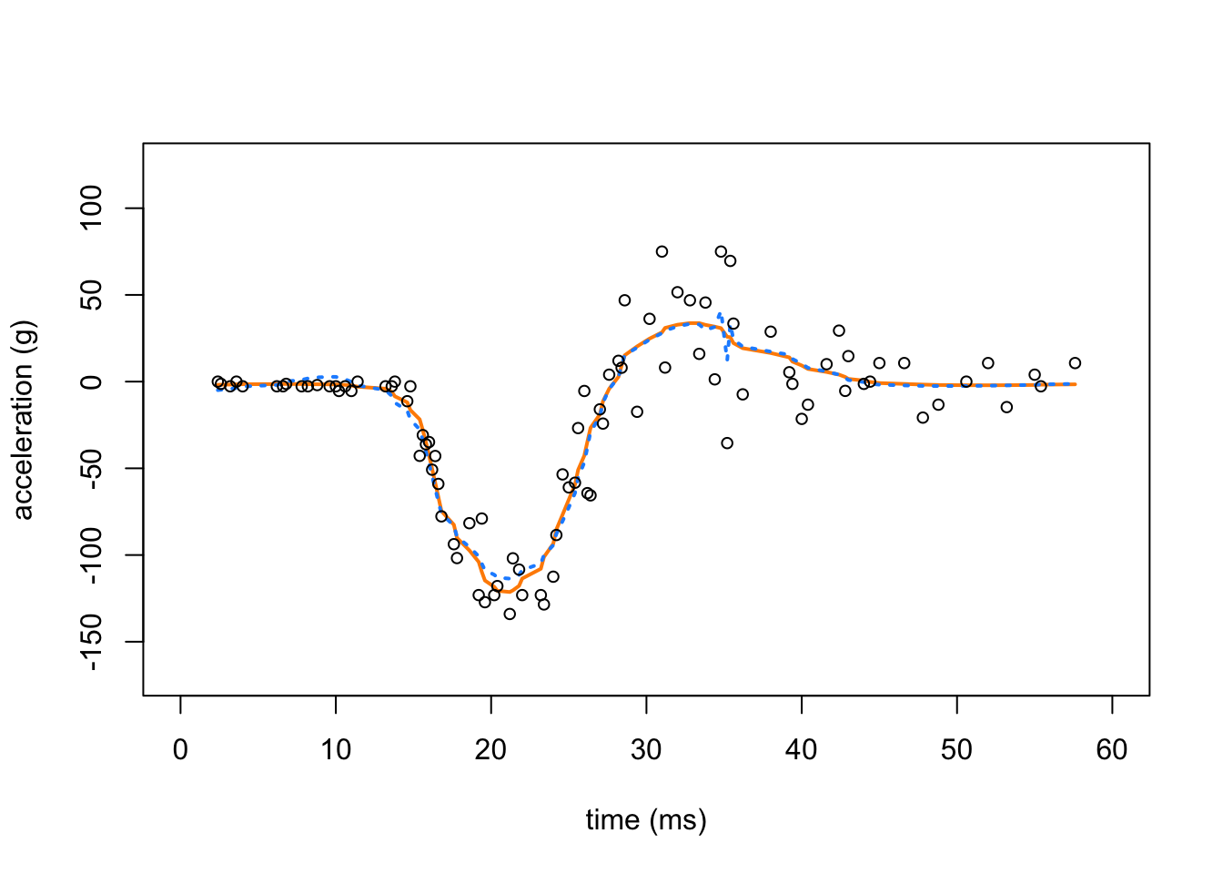
Expand here to see past versions of plot-homo-smash-estimates-1.png:
| Version | Author | Date |
|---|---|---|
| 3ce045f | Peter Carbonetto | 2018-11-06 |
And in this next plot, we compare the SMASH estimates (the orange line) against the the mean estimates obtained by TI thresholding (dark blue line), and TI thresholding when the variances have been estimated by SMASH (dotted green line).
plot(res.mc$x,res.mc$mu.est,type = "l",
     ylim = c(min(res.mc$y - 2 * sqrt(res.mc$var.est)),
              max(res.mc$y + 2 * sqrt(res.mc$var.est))),
     xlab = "time (ms)",ylab = "acceleration (g)",lwd = 2,
     col = "darkorange",xlim = c(0,60),xaxp = c(0,60,6))
lines(res.ti.cons.mc$x,res.ti.cons.mc$mu.est,lwd = 2,lty = "solid",
      col = "darkblue")
lines(res.ti.mc$x,res.ti.mc$mu.est,lwd = 2,col = "limegreen",lty = "dotted")
points(res.mc$x,res.mc$y,pch = 1,cex = 0.8,col = "black")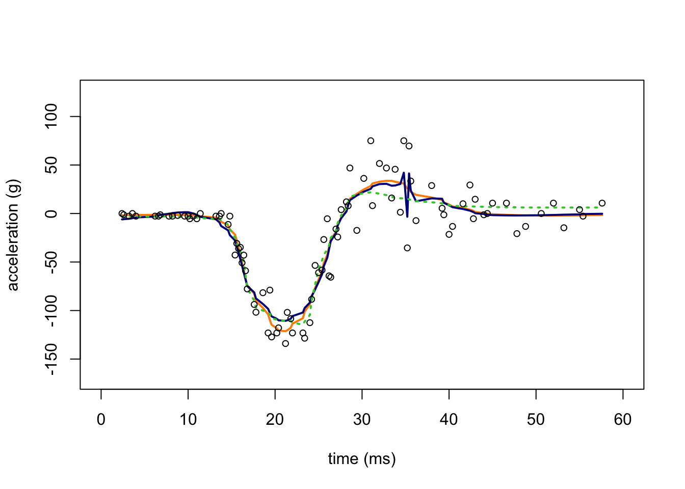
The TI thresholding estimate and the SMASH estimate with homoskedastic variances both show notable artifacts. When the TI thresholding method is provided with the SMASH variance estimate, the mean signal is substantially smoother.
Session information
sessionInfo()
# R version 3.4.3 (2017-11-30)
# Platform: x86_64-apple-darwin15.6.0 (64-bit)
# Running under: macOS High Sierra 10.13.6
#
# Matrix products: default
# BLAS: /Library/Frameworks/R.framework/Versions/3.4/Resources/lib/libRblas.0.dylib
# LAPACK: /Library/Frameworks/R.framework/Versions/3.4/Resources/lib/libRlapack.dylib
#
# locale:
# [1] en_US.UTF-8/en_US.UTF-8/en_US.UTF-8/C/en_US.UTF-8/en_US.UTF-8
#
# attached base packages:
# [1] stats     graphics  grDevices utils     datasets  methods   base
#
# other attached packages:
# [1] EbayesThresh_1.4-12 wavethresh_4.6.8    smashr_1.2-0
# [4] lattice_0.20-35     MASS_7.3-48
#
# loaded via a namespace (and not attached):
#  [1] Rcpp_1.0.0        knitr_1.20        whisker_0.3-2
#  [4] magrittr_1.5      workflowr_1.1.1   REBayes_1.3
#  [7] pscl_1.5.2        doParallel_1.0.11 SQUAREM_2017.10-1
# [10] foreach_1.4.4     ashr_2.2-23       stringr_1.3.1
# [13] caTools_1.17.1    tools_3.4.3       parallel_3.4.3
# [16] grid_3.4.3        data.table_1.11.4 R.oo_1.21.0
# [19] git2r_0.23.0      iterators_1.0.9   htmltools_0.3.6
# [22] assertthat_0.2.0  yaml_2.2.0        rprojroot_1.3-2
# [25] digest_0.6.17     Matrix_1.2-12     bitops_1.0-6
# [28] codetools_0.2-15  R.utils_2.6.0     evaluate_0.11
# [31] rmarkdown_1.10    stringi_1.2.4     compiler_3.4.3
# [34] Rmosek_8.0.69     backports_1.1.2   R.methodsS3_1.7.1
# [37] truncnorm_1.0-8
This reproducible R Markdown analysis was created with workflowr 1.1.1