Divvy usage over the year
Peter Carbonetto
Last updated: 2019-04-10
Checks: 6 0
Knit directory: wflow-divvy/analysis/
This reproducible R Markdown analysis was created with workflowr (version 1.2.0.9000). The Report tab describes the reproducibility checks that were applied when the results were created. The Past versions tab lists the development history.
Great! Since the R Markdown file has been committed to the Git repository, you know the exact version of the code that produced these results.
Great job! The global environment was empty. Objects defined in the global environment can affect the analysis in your R Markdown file in unknown ways. For reproduciblity it’s best to always run the code in an empty environment.
The command set.seed(1) was run prior to running the code in the R Markdown file. Setting a seed ensures that any results that rely on randomness, e.g. subsampling or permutations, are reproducible.
Great job! Recording the operating system, R version, and package versions is critical for reproducibility.
Nice! There were no cached chunks for this analysis, so you can be confident that you successfully produced the results during this run.
Great! You are using Git for version control. Tracking code development and connecting the code version to the results is critical for reproducibility. The version displayed above was the version of the Git repository at the time these results were generated.
Note that you need to be careful to ensure that all relevant files for the analysis have been committed to Git prior to generating the results (you can use wflow_publish or wflow_git_commit). workflowr only checks the R Markdown file, but you know if there are other scripts or data files that it depends on. Below is the status of the Git repository when the results were generated:
Ignored files:
    Ignored:    .DS_Store
    Ignored:    analysis/.DS_Store
    Ignored:    data/Divvy_Stations_2016_Q1Q2.csv
    Ignored:    data/Divvy_Stations_2016_Q3.csv
    Ignored:    data/Divvy_Stations_2016_Q4.csv
    Ignored:    data/Divvy_Trips_2016_04.csv
    Ignored:    data/Divvy_Trips_2016_05.csv
    Ignored:    data/Divvy_Trips_2016_06.csv
    Ignored:    data/Divvy_Trips_2016_Q1.csv
    Ignored:    data/Divvy_Trips_2016_Q3.csv
    Ignored:    data/Divvy_Trips_2016_Q4.csv
    Ignored:    data/README.txt
    Ignored:    data/data.tar.gz
    Ignored:    docs/.DS_Store
Note that any generated files, e.g. HTML, png, CSS, etc., are not included in this status report because it is ok for generated content to have uncommitted changes.
These are the previous versions of the R Markdown and HTML files. If you’ve configured a remote Git repository (see ?wflow_git_remote), click on the hyperlinks in the table below to view them.
| File | Version | Author | Date | Message |
|---|---|---|---|---|
| Rmd | 61c85b2 | Peter Carbonetto | 2019-04-10 | wflow_publish(c(“seasonal-trends.Rmd”, “station-map.Rmd”, |
| html | 54fcf4e | Peter Carbonetto | 2018-04-14 | Re-built station-map, time-of-day-trends and seasonal-trends webpages |
| Rmd | f163fe4 | Peter Carbonetto | 2018-04-14 | Updates for new workflowr version, v0.11.0.9000. |
| html | f163fe4 | Peter Carbonetto | 2018-04-14 | Updates for new workflowr version, v0.11.0.9000. |
| html | 51163d7 | Peter Carbonetto | 2018-03-12 | Ran wflow_publish(“*.Rmd“) with version v0.11.0 of workflowr. |
| html | ab9176e | Peter Carbonetto | 2018-03-09 | Added code_hiding to the analysis R Markdown files. |
| html | b32e833 | Peter Carbonetto | 2018-01-18 | Re-built all webpages using workflowr v0.1.0. |
| html | 93a3a86 | Peter Carbonetto | 2017-11-16 | Re-built seasonal-trends.html using workflowr v0.8.0. |
| Rmd | 5b8e33f | Peter Carbonetto | 2017-11-16 | wflow_publish(“seasonal-trends.Rmd”) |
| Rmd | 6b9ddf1 | Peter Carbonetto | 2017-08-02 | Added header with between-section spacing adjustment, and removed <br> tags from R Markdown files. |
| Rmd | c6e8686 | Peter Carbonetto | 2017-07-31 | wflow_publish(Sys.glob(“*.Rmd“)) |
| html | 727b8d9 | Peter Carbonetto | 2017-07-13 | Re-built all the analysis files; wflow_publish(Sys.glob(“*.Rmd“)). |
| Rmd | 6d02ffc | Peter Carbonetto | 2017-07-13 | Made a dozen or so small adjustments to the .Rmd files. |
| html | bf818d8 | Peter Carbonetto | 2017-07-07 | Ran wflow_publish(c(“index.Rmd”, “setup.Rmd”, “station-map.Rmd”, |
| Rmd | e4ba033 | Peter Carbonetto | 2017-07-07 | Removed use of word ‘notebook’. |
| html | cbee77b | Peter Carbonetto | 2017-07-07 | Ran wflow_publish(seasonal-trends.Rmd). |
| Rmd | 984143c | Peter Carbonetto | 2017-07-07 | Made a few small revisions to seasonal-trends.Rmd. |
| html | 34518f3 | Peter Carbonetto | 2017-07-06 | Built first draft of seasonal trends notebook. |
| Rmd | 6ef7a6c | Peter Carbonetto | 2017-07-06 | wflow_publish(“seasonal-trends.Rmd”) |
| Rmd | c8f7e10 | Peter Carbonetto | 2017-07-06 | Implemented first draft of seasonal trends notebook. |
In this last analysis, I use the Divvy trip data to examine biking trends in Chicago over the course of one year.
I begin by loading a few packages, as well as some additional functions I wrote for this project.
library(data.table)
library(ggplot2)
source("../code/functions.R")
Read the data
First, I read in the Divvy trip and station data from the CSV files.
divvy <- read.divvy.data()
# Reading station data from ../data/Divvy_Stations_2016_Q4.csv.
# Reading trip data from ../data/Divvy_Trips_2016_Q1.csv.
# Reading trip data from ../data/Divvy_Trips_2016_04.csv.
# Reading trip data from ../data/Divvy_Trips_2016_05.csv.
# Reading trip data from ../data/Divvy_Trips_2016_06.csv.
# Reading trip data from ../data/Divvy_Trips_2016_Q3.csv.
# Reading trip data from ../data/Divvy_Trips_2016_Q4.csv.
# Preparing Divvy data for analysis in R.
# Converting dates and times.
I would like to analyze city-wide departures for each day of the year, so I create a new “day of year” column.
divvy$trips <-
  transform(divvy$trips,
    start.dayofyear = factor(as.numeric(format(divvy$trips$starttime,"%j")),
                             1:366))
I also convert the “start week” column to a factor to make it easier to compile trip statistics for each week in the year.
divvy$trips <- transform(divvy$trips,start.week = factor(start.week,0:52))Plot departures per day and per week
Here, I create a new vector containing the number of trips taken in each day of the year, and then I plot these numbers.
counts.day <- as.vector(table(divvy$trips$start.dayofyear))
ggplot(data.frame(day = 1:366,departures = counts.day),
       aes(x = day,y = departures)) +
  geom_point(color = "darkblue",shape = 19,size = 1) +
  geom_line(color = "darkblue") +
  scale_x_continuous(breaks = seq(0,350,25)) +
  theme_minimal() +
  theme(panel.grid.major = element_blank(),
        panel.grid.minor = element_blank())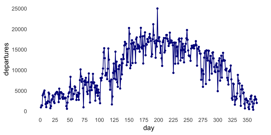
This plot shows a sizeable increase in bike trips during summer days, but since the number of trips varies widely from one day to the next, I think the plot will look nicer if instead we count the number of trips per week.
counts.week <- as.vector(table(divvy$trips$start.week))
ggplot(data.frame(week = 0:52,departures = counts.week),
       aes(x = week,y = departures)) +
  geom_point(color = "darkblue",shape = 19,size = 1.5) +
  geom_line(color = "darkblue") +
  theme_minimal() +
  theme(panel.grid.major = element_blank(),
        panel.grid.minor = element_blank())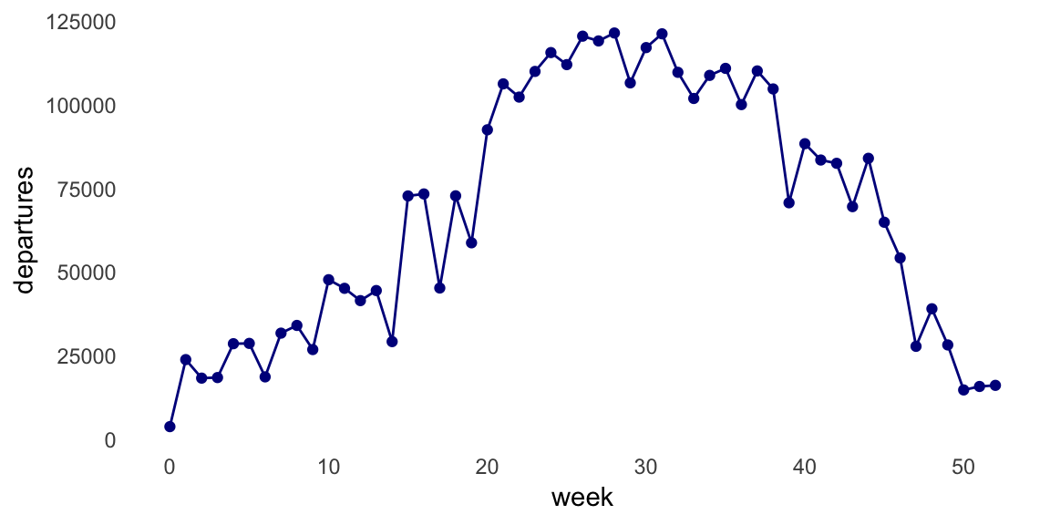
Indeed, the seasonal trends are less noisy in this plot; the majority of Divvy bike trips in Chicago are taken when the weather is warmer (weeks 20–40), and very few people are using the Divvy bikes in the cold winter months.
Seasonal trends at the University of Chicago
When we analyze trips taken at the University of Chicago bike station, the “bump” during warmer months flattens out. This is probably because a large fraction of University of Chicago students leave during the summer.
dat <- subset(divvy$trips,from_station_name == "University Ave & 57th St")
counts.week.uchicago <- as.vector(table(dat$start.week))
ggplot(data.frame(week = 0:52,departures = counts.week.uchicago),
       aes(x = week,y = departures)) +
  geom_point(color = "darkblue",shape = 19,size = 1.5) +
  geom_line(color = "darkblue") +
  theme_minimal() +
  theme(panel.grid.major = element_blank(),
        panel.grid.minor = element_blank())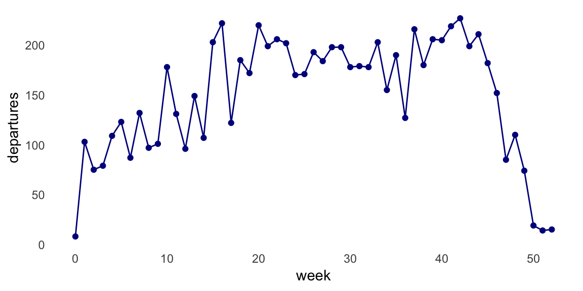
This is the version of R and the packages that were used to generate these results.
sessionInfo()
# R version 3.4.3 (2017-11-30)
# Platform: x86_64-apple-darwin15.6.0 (64-bit)
# Running under: macOS High Sierra 10.13.6
#
# Matrix products: default
# BLAS: /Library/Frameworks/R.framework/Versions/3.4/Resources/lib/libRblas.0.dylib
# LAPACK: /Library/Frameworks/R.framework/Versions/3.4/Resources/lib/libRlapack.dylib
#
# locale:
# [1] en_US.UTF-8/en_US.UTF-8/en_US.UTF-8/C/en_US.UTF-8/en_US.UTF-8
#
# attached base packages:
# [1] stats     graphics  grDevices utils     datasets  methods   base
#
# other attached packages:
# [1] ggplot2_3.1.0     data.table_1.11.4
#
# loaded via a namespace (and not attached):
#  [1] Rcpp_1.0.0           knitr_1.20           whisker_0.3-2
#  [4] magrittr_1.5         workflowr_1.2.0.9000 tidyselect_0.2.5
#  [7] munsell_0.4.3        colorspace_1.4-0     R6_2.2.2
# [10] rlang_0.3.1          dplyr_0.8.0.1        stringr_1.3.1
# [13] plyr_1.8.4           tools_3.4.3          grid_3.4.3
# [16] gtable_0.2.0         withr_2.1.2          git2r_0.23.3
# [19] htmltools_0.3.6      assertthat_0.2.0     yaml_2.2.0
# [22] lazyeval_0.2.1       rprojroot_1.3-2      digest_0.6.17
# [25] tibble_2.1.1         crayon_1.3.4         purrr_0.2.5
# [28] fs_1.2.6             glue_1.3.0           evaluate_0.11
# [31] rmarkdown_1.10       labeling_0.3         stringi_1.2.4
# [34] pillar_1.3.1         compiler_3.4.3       scales_0.5.0
# [37] backports_1.1.2      pkgconfig_2.0.2