Sample Collection Distribution
Juan Manuel Vazquez
2022-11-08
Last updated: 2023-10-23
Checks: 5 1
Knit directory: R_workflowr/analysis/
This reproducible R Markdown analysis was created with workflowr (version 1.7.1). The Checks tab describes the reproducibility checks that were applied when the results were created. The Past versions tab lists the development history.
Great job! The global environment was empty. Objects defined in the global environment can affect the analysis in your R Markdown file in unknown ways. For reproduciblity it’s best to always run the code in an empty environment.
The command set.seed(20230501) was run prior to running
the code in the R Markdown file. Setting a seed ensures that any results
that rely on randomness, e.g. subsampling or permutations, are
reproducible.
Great job! Recording the operating system, R version, and package versions is critical for reproducibility.
Nice! There were no cached chunks for this analysis, so you can be confident that you successfully produced the results during this run.
Great job! Using relative paths to the files within your workflowr project makes it easier to run your code on other machines.
Tracking code development and connecting the code version to the
results is critical for reproducibility. To start using Git, open the
Terminal and type git init in your project directory.
This project is not being versioned with Git. To obtain the full
reproducibility benefits of using workflowr, please see
?wflow_start.
our_genomes = c(
  "Myotis_auriculus",
  "Myotis_californicus",
  "Myotis_occultus",
  "Myotis_lucifugus",
  "Myotis_yumanensis",
  "Myotis_volans",
  "Myotis_velifer",
  "Myotis_evotis",
  "Myotis_thysanodes"
)

species_color = ggsci::pal_d3(palette = "category20")(length(our_genomes)+1) %>%
  set_names(., c(our_genomes, "Other"))
species_color["Myotis_evotis"] = "#17BECFFF"
species_color["Other"] = "#7F7F7FFF"
sheet_cols <- c(
'CollectionID' = 'c',
'Source Info & Permit #' = 'c',
'Date Captured' = 'D',
'Date Sampled' = 'D',
'SampleTimeStart' = 't',
'SampleTimeEnd' = 't',
'Collector' = 'c',
'County' = 'c',
'State' = 'c',
'LocationShort' = 'c',
'LocationFull' = 'c',
'LocationDetails' = 'c',
'CoordExact' = 'c',
'What3Words' = 'c',
'Lattitude' = 'd',
'Longitude' = 'd',
'Altitude (ft)' = 'c',
'Net #' = 'c',
'FieldSpeciesID' = 'c',
'FieldSpeciesMethod' = 'c',
'ConfirmedSpeciesID' = 'c',
'ConfirmationMethod' = 'c',
'Sex' = 'c',
'Age' = 'c',
'Reproductive Status' = 'c',
'Weight (g)' = 'd',
'Forearm (mm)' = 'd',
'Ear (mm)' = 'd',
'Tragus (mm)' = 'd',
'Tail (mm)' = 'd',
'Thumb (mm)' = 'd',
'WNS Status' = 'c',
'HasAccoustic' = 'c',
'PunchesCollected' = 'c',
'Preservation' = 'c',
'OtherSamples' = 'c',
'OtherMeasurements' = 'c',
'Comments' = 'c',
'AltID' = 'c'
)
# datasheet <- read_sheet("https://docs.google.com/spreadsheets/d/1DJctPKAd9TQOLNnmGXP8t0TPAEe4-CICus9QZ7IYsCU/edit#gid=915133740", col_types = sheet_cols %>% paste0(collapse=""))
# datasheet %>% write_tsv("../data/collection_datasheet_2022-11-15.tsv")
datasheet <- read_tsv("../data/collection_datasheet_2022-11-15.tsv", col_types = sheet_cols %>% paste0(collapse=""))shape.myoAui <- dir(path="../data/USGS_SpeciesRanges/Myotis_auriculus/", pattern = ".shp$", full.names=T) %>%
st_read() %>%
mutate(species = "Myotis_auriculus") %>%
st_make_valid()
shape.myoCai <- dir(path = "../data/USGS_SpeciesRanges/Myotis_californicus/", pattern = ".shp$", full.names=T) %>%
st_read() %>%
mutate(species = "Myotis_californicus") %>%
st_make_valid()
shape.myoOcc <- dir(path = "../data/USGS_SpeciesRanges/Myotis_occultus/", pattern = ".shp$", full.names=T) %>%
st_read() %>%
mutate(species = "Myotis_occultus") %>%
st_make_valid()
shape.myoLuc <- dir(path = "../data/USGS_SpeciesRanges/Myotis_lucifugus/", pattern = ".shp$", full.names=T) %>%
st_read() %>%
mutate(species = "Myotis_lucifugus") %>%
st_make_valid()
shape.myoYum <- dir(path = "../data/USGS_SpeciesRanges/Myotis_yumanensis/", pattern = ".shp$", full.names=T) %>%
st_read() %>%
mutate(species = "Myotis_yumanensis") %>%
st_make_valid()
shape.myoVol <- dir(path = "../data/USGS_SpeciesRanges/Myotis_volans/", pattern = ".shp$", full.names=T) %>%
st_read() %>%
mutate(species = "Myotis_volans") %>%
st_make_valid()
shape.myoVel <- dir(path = "../data/USGS_SpeciesRanges/Myotis_velifer/", pattern = ".shp$", full.names=T) %>%
st_read() %>%
mutate(species = "Myotis_velifer") %>%
st_make_valid()
shape.myoEvo <- dir(path = "../data/USGS_SpeciesRanges/Myotis_evotis/", pattern = ".shp$", full.names=T) %>%
st_read() %>%
mutate(species = "Myotis_evotis") %>%
st_make_valid()
shape.myoThy <- dir(path = "../data/USGS_SpeciesRanges/Myotis_thysanodes/", pattern = ".shp$", full.names=T) %>%
st_read() %>%
mutate(species = "Myotis_thysanodes") %>%
st_make_valid()world <- ne_countries(scale = "medium", returnclass = "sf") %>%
st_make_valid()
northAmerica <- ne_countries(scale = "medium", returnclass = "sf", country = c("United States of America", "Mexico", "Canada")) %>% st_make_valid
# class(world)
states <- st_as_sf(map("state", plot = FALSE, fill = TRUE))
west <- subset(states, ID %in% c("california", "arizona", "nevada", "new mexico", "idaho", "oregon", "washington", "montana", "nebraska", "colorado", "utah", "wyoming"))
notwest <- subset(states, !(ID %in% c("california", "arizona", "nevada", "new mexico", "idaho", "oregon", "washington", "montana", "nebraska", "colorado", "utah", "wyoming")))
cal <- subset(states, ID == "california")
calaz <- subset(states, ID %in% c("california", "arizona"))
caaznv <- subset(states, ID %in% c("california", "arizona", "nevada"))
notcalaz <- subset(states, !(ID %in% c("california", "arizona")))datasheet.known <- datasheet %>%
filter(!is.na(Lattitude)) %>%
select(species=FieldSpeciesID, Lattitude, Longitude) #%>%
# mutate(species = species %>% str_replace_all(" ", "_"))
p.map.collections <- ggplot() +
geom_sf(data= west, color = "#ABB0B8", fill = "#6F7378", size = 0.1) +
geom_spatial_point(data= datasheet.known, aes(group=species, y=Lattitude, x=Longitude, color=species), size=4, position="jitter") +
geom_spatial_label_repel(data= datasheet.known, aes(label=species,group=species, y=Lattitude, x=Longitude, color=species), show.legend=F) +
scale_color_manual(values = species_color %>% set_names(., names(.) %>% str_replace_all("_", " "))) +
ggpubr::theme_pubclean() +
theme(legend.position = "none")
p.map.collectionsAssuming `crs = 4326` in stat_spatial_identity()
Assuming `crs = 4326` in stat_spatial_identity()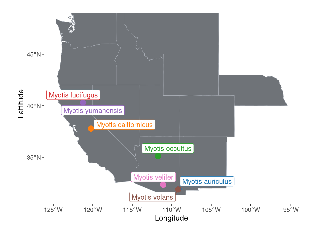
p.map.collections.caaznv <- ggplot() +
  geom_sf(data= caaznv, color = "#ABB0B8", fill = "#6F7378", size = 0.1) +
  geom_spatial_point(data= datasheet.known, aes(group=species, y=Lattitude, x=Longitude, fill=species), size=4, pch=21, position="jitter") +
  geom_spatial_label_repel(data= datasheet.known, aes(label=species,group=species, y=Lattitude, x=Longitude, fill=species), show.legend=F, color='black', nudge_x=-0.5) +
  scale_color_manual(values = species_color %>% set_names(., names(.) %>% str_replace_all("_", " "))) +
  scale_fill_manual(values = species_color %>% set_names(., names(.) %>% str_replace_all("_", " "))) +
  ggpubr::theme_pubclean() +
  theme(legend.position = "none")

p.map.collections.caaznv
Assuming `crs = 4326` in stat_spatial_identity()
Assuming `crs = 4326` in stat_spatial_identity()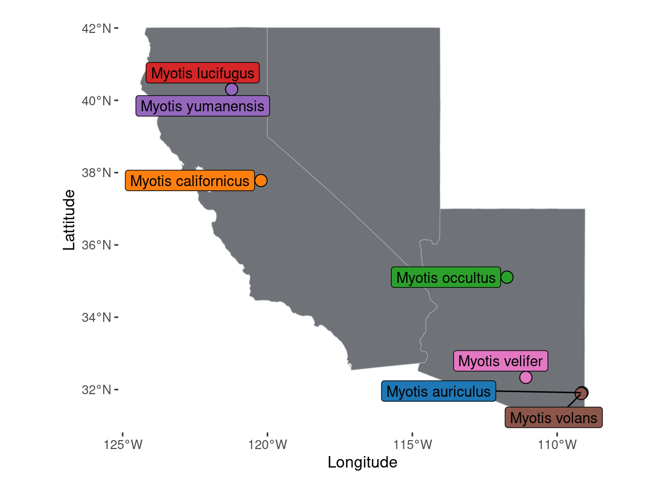
shape.myoLuc$geometry <- shape.myoLuc$geometry %>%
  s2::s2_rebuild() %>%
  sf::st_as_sfc()
sf::sf_use_s2(TRUE)
st_intersection(west, shape.myoLuc)
shape.myoLuc2 <- st_transform(shape.myoLuc, "NAD83")
st_crs(shape.myoLuc)
st_crs(shape.myoLuc2)
st_crs(west)
west2 <- st_transform(west, crs="NAD83")
st_crs(west2)
shape.myoLuc3 <- shape.myoLuc
st_crs(shape.myoLuc3) <- "NAD83"
st_intersection(shape.myoLuc3, west2)
p.mapMyo.split <- ggplot() +
geom_sf(data= west, color = "#ABB0B8", fill = "#6F7378", size = 0.1) +
annotation_spatial(data = shape.myoLuc, aes(group = species, fill=species), alpha = 0.8, color="black") +
annotation_spatial(data = shape.myoYum, aes(group = species, fill=species), alpha = 0.8, color="black") +
annotation_spatial(data = shape.myoCai, aes(group = species, fill=species), alpha = 0.8, color="black") +
annotation_spatial(data = shape.myoVol, aes(group = species, fill=species), alpha = 0.8, color="black") +
annotation_spatial(data = shape.myoEvo, aes(group = species, fill=species), alpha = 0.8, color="black") +
annotation_spatial(data = shape.myoThy, aes(group = species, fill=species), alpha = 0.8, color="black") +
annotation_spatial(data = shape.myoOcc, aes(group = species, fill=species), alpha = 0.8, color="black") +
annotation_spatial(data = shape.myoVel, aes(group = species, fill=species), alpha = 0.8, color="black") +
annotation_spatial(data = shape.myoAui, aes(group = species, fill=species), alpha = 0.8, color="black") +
annotation_spatial(data=notwest, fill="white", color="white") +
geom_spatial_point(data= datasheet.known, aes(group=species, y=Lattitude, x=Longitude), size=2) +
scale_fill_manual("Species", values = species_color) +
scale_color_manual("Species", values = species_color) +
guides(fill=guide_none()) +
theme_void() +
facet_wrap(~species) +
theme(
strip.text = element_text(face="bold", size=12, hjust = 0.5)
)
p.mapMyo.splitAssuming `crs = 4326` in stat_spatial_identity()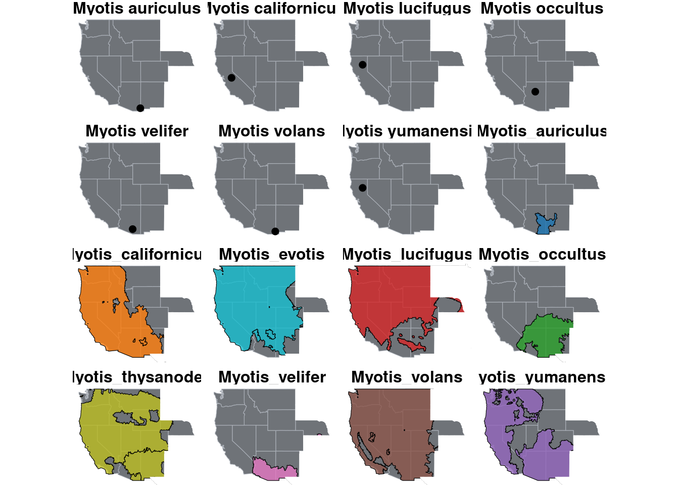
#%>% plotly::ggplotly()pic.myoLuc <- image_read("https://www.batcon.org/wp-content/uploads/2020/02/108746-19-e1593640880404.jpg") %>% image_ggplot()
pic.myoYum <- image_read("https://www.batcon.org/wp-content/uploads/2020/02/106605-56-812x600.jpg") %>% image_ggplot()
pic.myoCai <- image_read("https://www.batcon.org/wp-content/uploads/2020/02/106608-56-812x600.jpg") %>% image_ggplot()
pic.myoVol <- image_read("https://www.batcon.org/wp-content/uploads/2020/02/106442-19-812x600.jpg") %>% image_ggplot()
pic.myoEvo <- image_read("https://www.batcon.org/wp-content/uploads/2020/02/Long-eared-Myotis-MYOTIS-EVOTIS-Michael-DurhamMinden-PIctures-e1642201106124-812x600.jpeg") %>% image_ggplot()
pic.myoThy <- image_read("https://www.batcon.org/wp-content/uploads/2020/02/106472-19.jpg") %>% image_ggplot()
pic.myoOcc <- image_read("https://www.batcon.org/wp-content/uploads/2020/02/Arizona-myotis-Rick-and-Nora-Bowers-Alamy-Stock-Photo--812x600.jpeg") %>% image_ggplot()
pic.myoVel <- image_read("https://www.batcon.org/wp-content/uploads/2020/02/106463-19-e1642201625671-812x600.jpg") %>% image_ggplot()
pic.myoAui <- image_read("https://www.batcon.org/wp-content/uploads/2020/02/106475-19-e1593638188243-812x600.jpg") %>% image_ggplot()p.map.base <- ggplot() +
geom_sf(data= west, color = "#ABB0B8", fill = "#6F7378", size = 0.1)
p.map.myoLuc <- p.map.base +
annotation_spatial(data = shape.myoLuc, aes(group = species, fill=species), alpha = 0.8, color="black") +
annotation_spatial(data=notwest, fill="white", color="white") +
scale_fill_manual(values = species_color) +
guides(fill=guide_none()) +
theme_void() +
theme(title = element_text(face="bold", size=12, hjust = 0.5),
plot.background = element_rect(color="black"),
plot.margin = margin(0,0,0,0, "cm")) +
ggtitle("Myotis lucifugus") +
geom_spatial_point(data= datasheet.known %>% filter(species == "Myotis_lucifugus"), aes(group=species, y=Lattitude, x=Longitude), size=2)
p.map.myoYum <- p.map.base +
annotation_spatial(data = shape.myoYum, aes(group = species, fill=species), alpha = 0.8, color="black") +
annotation_spatial(data=notwest, fill="white", color="white") +
scale_fill_manual(values = species_color) +
guides(fill=guide_none()) +
theme_void() +
theme(title = element_text(face="bold", size=12, hjust = 0.5),
plot.background = element_rect(color="black"),
plot.margin = margin(0,0,0,0, "cm")) +
ggtitle("Myotis yumanensis") +
geom_spatial_point(data= datasheet.known %>% filter(species == "Myotis_yumanensis"), aes(group=species, y=Lattitude, x=Longitude), size=2)
p.map.myoCai <- p.map.base +
annotation_spatial(data = shape.myoCai, aes(group = species, fill=species), alpha = 0.8, color="black") +
annotation_spatial(data=notwest, fill="white", color="white") +
scale_fill_manual(values = species_color) +
guides(fill=guide_none()) +
theme_void() +
theme(title = element_text(face="bold", size=12, hjust = 0.5),
plot.background = element_rect(color="black"),
plot.margin = margin(0,0,0,0, "cm")) +
ggtitle("Myotis californicus") +
geom_spatial_point(data= datasheet.known %>% filter(species == "Myotis_californicus"), aes(group=species, y=Lattitude, x=Longitude), size=2)
p.map.myoVol <- p.map.base +
annotation_spatial(data = shape.myoVol, aes(group = species, fill=species), alpha = 0.8, color="black") +
annotation_spatial(data=notwest, fill="white", color="white") +
scale_fill_manual(values = species_color) +
guides(fill=guide_none()) +
theme_void() +
theme(title = element_text(face="bold", size=12, hjust = 0.5),
plot.background = element_rect(color="black"),
plot.margin = margin(0,0,0,0, "cm")) +
ggtitle("Myotis volans") +
geom_spatial_point(data= datasheet.known %>% filter(species == "Myotis_volans"), aes(group=species, y=Lattitude, x=Longitude), size=2)
p.map.myoEvo <- p.map.base +
annotation_spatial(data = shape.myoEvo, aes(group = species, fill=species), alpha = 0.8, color="black") +
annotation_spatial(data=notwest, fill="white", color="white") +
scale_fill_manual(values = species_color) +
guides(fill=guide_none()) +
theme_void() +
theme(title = element_text(face="bold", size=12, hjust = 0.5),
plot.background = element_rect(color="black"),
plot.margin = margin(0,0,0,0, "cm")) +
ggtitle("Myotis evotis") +
geom_spatial_point(data= datasheet.known %>% filter(species == "Myotis_evotis"), aes(group=species, y=Lattitude, x=Longitude), size=2)
p.map.myoThy <- p.map.base +
annotation_spatial(data = shape.myoThy, aes(group = species, fill=species), alpha = 0.8, color="black") +
annotation_spatial(data=notwest, fill="white", color="white") +
scale_fill_manual(values = species_color) +
guides(fill=guide_none()) +
theme_void() +
theme(title = element_text(face="bold", size=12, hjust = 0.5),
plot.background = element_rect(color="black"),
plot.margin = margin(0,0,0,0, "cm")) +
ggtitle("Myotis thysanodes") +
geom_spatial_point(data= datasheet.known %>% filter(species == "Myotis_thysanodes"), aes(group=species, y=Lattitude, x=Longitude), size=2)
p.map.myoOcc <- p.map.base +
annotation_spatial(data = shape.myoOcc, aes(group = species, fill=species), alpha = 0.8, color="black") +
annotation_spatial(data=notwest, fill="white", color="white") +
scale_fill_manual(values = species_color) +
guides(fill=guide_none()) +
theme_void() +
theme(title = element_text(face="bold", size=12, hjust = 0.5),
plot.background = element_rect(color="black"),
plot.margin = margin(0,0,0,0, "cm")) +
ggtitle("Myotis occultus") +
geom_spatial_point(data= datasheet.known %>% filter(species == "Myotis_occultus"), aes(group=species, y=Lattitude, x=Longitude), size=2)
p.map.myoVel <- p.map.base +
annotation_spatial(data = shape.myoVel, aes(group = species, fill=species), alpha = 0.8, color="black") +
annotation_spatial(data=notwest, fill="white", color="white") +
scale_fill_manual(values = species_color) +
guides(fill=guide_none()) +
theme_void() +
theme(title = element_text(face="bold", size=12, hjust = 0.5),
plot.background = element_rect(color="black"),
plot.margin = margin(0,0,0,0, "cm")) +
ggtitle("Myotis velifer") +
geom_spatial_point(data= datasheet.known %>% filter(species == "Myotis_velifer"), aes(group=species, y=Lattitude, x=Longitude), size=2)
p.map.myoAui <- p.map.base +
annotation_spatial(data = shape.myoAui, aes(group = species, fill=species), alpha = 0.8, color="black") +
annotation_spatial(data=notwest, fill="white", color="white") +
scale_fill_manual(values = species_color) +
guides(fill=guide_none()) +
theme_void() +
theme(title = element_text(face="bold", size=12, hjust = 0.5),
plot.background = element_rect(color="black"),
plot.margin = margin(0,0,0,0, "cm")) +
ggtitle("Myotis auriculus") +
geom_spatial_point(data= datasheet.known %>% filter(species == "Myotis_auriculus"), aes(group=species, y=Lattitude, x=Longitude), size=2)
p.map.pic.myoLuc <- p.map.myoLuc + inset_element(pic.myoLuc, left = 0.69, bottom = 0.6, right = 1, top = 1)
p.map.pic.myoYum <- p.map.myoYum + inset_element(pic.myoYum, left = 0.69, bottom = 0.6, right = 1, top = 1)
p.map.pic.myoCai <- p.map.myoCai + inset_element(pic.myoCai, left = 0.69, bottom = 0.6, right = 1, top = 1)
p.map.pic.myoVol <- p.map.myoVol + inset_element(pic.myoVol, left = 0.69, bottom = 0.6, right = 1, top = 1)
p.map.pic.myoEvo <- p.map.myoEvo + inset_element(pic.myoEvo, left = 0.69, bottom = 0.6, right = 1, top = 1)
p.map.pic.myoThy <- p.map.myoThy + inset_element(pic.myoThy, left = 0.69, bottom = 0.6, right = 1, top = 1)
p.map.pic.myoOcc <- p.map.myoOcc + inset_element(pic.myoOcc, left = 0.69, bottom = 0.6, right = 1, top = 1)
p.map.pic.myoVel <- p.map.myoVel + inset_element(pic.myoVel, left = 0.69, bottom = 0.6, right = 1, top = 1)
p.map.pic.myoAui <- p.map.myoAui + inset_element(pic.myoAui, left = 0.69, bottom = 0.6, right = 1, top = 1)
p.mapPic <- (p.map.pic.myoLuc | p.map.pic.myoYum | p.map.pic.myoCai)/
(p.map.pic.myoVol | p.map.pic.myoEvo | p.map.pic.myoThy)/
(p.map.pic.myoOcc | p.map.pic.myoVel | p.map.pic.myoAui)
p.mapPic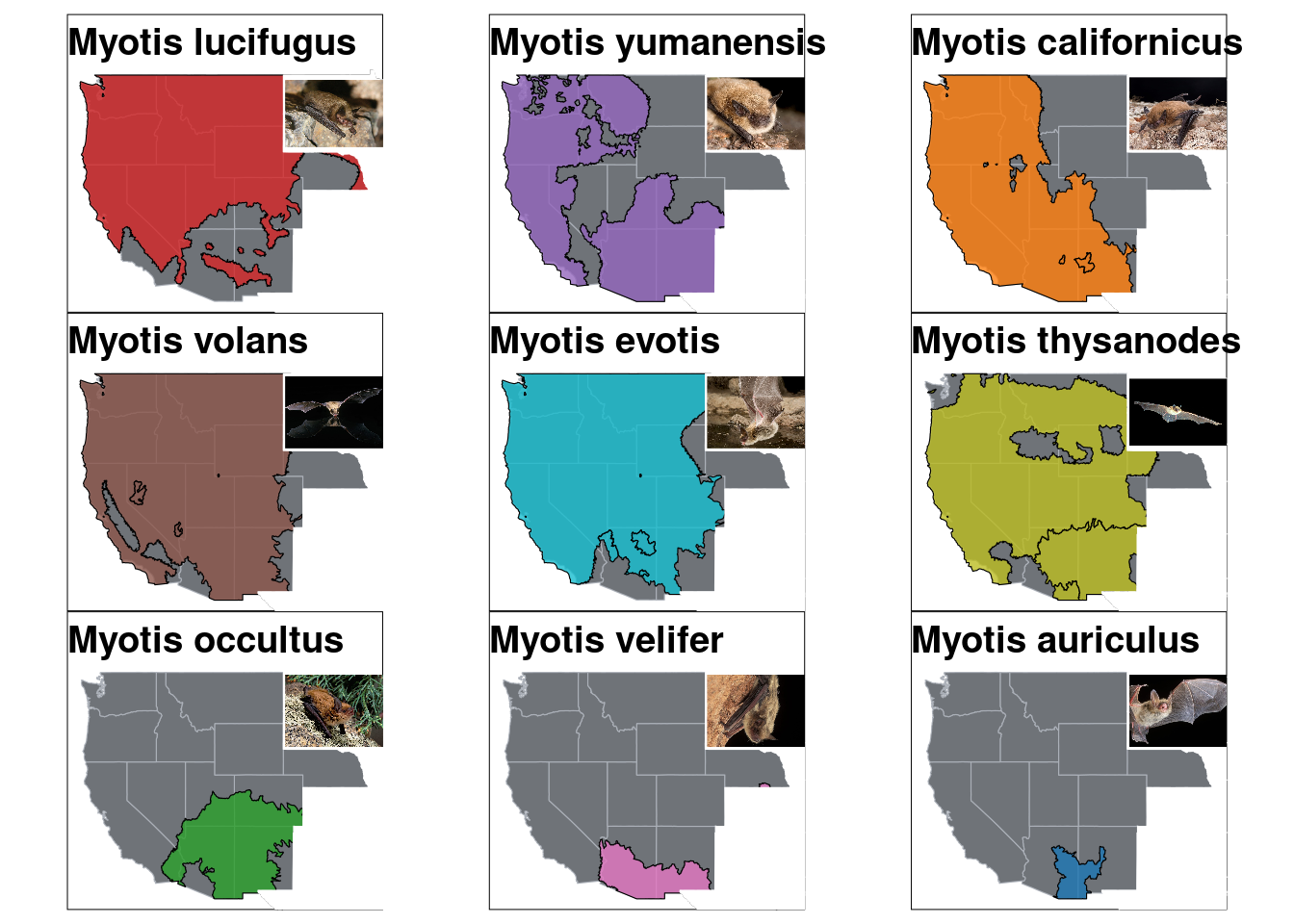
p.map.base.calaz <- ggplot() +
  geom_sf(data= calaz, color = "#ABB0B8", fill = "#6F7378", size = 0.1)

p.map.myoLuc.calaz <- p.map.base.calaz +
  annotation_spatial(data = shape.myoLuc, aes(group = species, fill=species), alpha = 0.8, color="black") +
  annotation_spatial(data=notcalaz, fill="white", color="white") +
  scale_fill_manual(values = species_color) +
  guides(fill=guide_none()) +
  theme_void() +
  theme(title = element_text(face="bold", size=12, hjust = 0.5), plot.margin = margin(0,0,0,0, "cm")) +
  ggtitle("Myotis lucifugus") +
  geom_spatial_point(data= datasheet.known %>% filter(species == "Myotis_lucifugus"), aes(group=species, y=Lattitude, x=Longitude), size=2)
p.map.myoYum.calaz <- p.map.base.calaz +
  annotation_spatial(data = shape.myoYum, aes(group = species, fill=species), alpha = 0.8, color="black") +
  annotation_spatial(data=notcalaz, fill="white", color="white") +
  scale_fill_manual(values = species_color) +
  guides(fill=guide_none()) +
  theme_void() +
  theme(title = element_text(face="bold", size=12, hjust = 0.5), plot.margin = margin(0,0,0,0, "cm")) +
  ggtitle("Myotis yumanensis") +
  geom_spatial_point(data= datasheet.known %>% filter(species == "Myotis_yumanensis"), aes(group=species, y=Lattitude, x=Longitude), size=2)
p.map.myoCai.calaz <- p.map.base.calaz +
  annotation_spatial(data = shape.myoCai, aes(group = species, fill=species), alpha = 0.8, color="black") +
  annotation_spatial(data=notcalaz, fill="white", color="white") +
  scale_fill_manual(values = species_color) +
  guides(fill=guide_none()) +
  theme_void() +
  theme(title = element_text(face="bold", size=12, hjust = 0.5), plot.margin = margin(0,0,0,0, "cm")) +
  ggtitle("Myotis californicus") +
  geom_spatial_point(data= datasheet.known %>% filter(species == "Myotis_californicus"), aes(group=species, y=Lattitude, x=Longitude), size=2)
p.map.myoVol.calaz <- p.map.base.calaz +
  annotation_spatial(data = shape.myoVol, aes(group = species, fill=species), alpha = 0.8, color="black") +
  annotation_spatial(data=notcalaz, fill="white", color="white") +
  scale_fill_manual(values = species_color) +
  guides(fill=guide_none()) +
  theme_void() +
  theme(title = element_text(face="bold", size=12, hjust = 0.5), plot.margin = margin(0,0,0,0, "cm")) +
  ggtitle("Myotis volans") +
  geom_spatial_point(data= datasheet.known %>% filter(species == "Myotis_volans"), aes(group=species, y=Lattitude, x=Longitude), size=2)
p.map.myoEvo.calaz <- p.map.base.calaz +
  annotation_spatial(data = shape.myoEvo, aes(group = species, fill=species), alpha = 0.8, color="black") +
  annotation_spatial(data=notcalaz, fill="white", color="white") +
  scale_fill_manual(values = species_color) +
  guides(fill=guide_none()) +
  theme_void() +
  theme(title = element_text(face="bold", size=12, hjust = 0.5), plot.margin = margin(0,0,0,0, "cm")) +
  ggtitle("Myotis evotis") +
  geom_spatial_point(data= datasheet.known %>% filter(species == "Myotis_evotis"), aes(group=species, y=Lattitude, x=Longitude), size=2)
p.map.myoThy.calaz <- p.map.base.calaz +
  annotation_spatial(data = shape.myoThy, aes(group = species, fill=species), alpha = 0.8, color="black") +
  annotation_spatial(data=notcalaz, fill="white", color="white") +
  scale_fill_manual(values = species_color) +
  guides(fill=guide_none()) +
  theme_void() +
  theme(title = element_text(face="bold", size=12, hjust = 0.5), plot.margin = margin(0,0,0,0, "cm")) +
  ggtitle("Myotis thysanodes") +
  geom_spatial_point(data= datasheet.known %>% filter(species == "Myotis_thysanodes"), aes(group=species, y=Lattitude, x=Longitude), size=2)
p.map.myoOcc.calaz <- p.map.base.calaz +
  annotation_spatial(data = shape.myoOcc, aes(group = species, fill=species), alpha = 0.8, color="black") +
  annotation_spatial(data=notcalaz, fill="white", color="white") +
  scale_fill_manual(values = species_color) +
  guides(fill=guide_none()) +
  theme_void() +
  theme(title = element_text(face="bold", size=12, hjust = 0.5), plot.margin = margin(0,0,0,0, "cm")) +
  ggtitle("Myotis occultus") +
  geom_spatial_point(data= datasheet.known %>% filter(species == "Myotis_occultus"), aes(group=species, y=Lattitude, x=Longitude), size=2)
p.map.myoVel.calaz <- p.map.base.calaz +
  annotation_spatial(data = shape.myoVel, aes(group = species, fill=species), alpha = 0.8, color="black") +
  annotation_spatial(data=notcalaz, fill="white", color="white") +
  scale_fill_manual(values = species_color) +
  guides(fill=guide_none()) +
  theme_void() +
  theme(title = element_text(face="bold", size=12, hjust = 0.5), plot.margin = margin(0,0,0,0, "cm")) +
  ggtitle("Myotis velifer") +
  geom_spatial_point(data= datasheet.known %>% filter(species == "Myotis_velifer"), aes(group=species, y=Lattitude, x=Longitude), size=2)
p.map.myoAui.calaz <- p.map.base.calaz +
  annotation_spatial(data = shape.myoAui, aes(group = species, fill=species), alpha = 0.8, color="black") +
  annotation_spatial(data=notcalaz, fill="white", color="white") +
  scale_fill_manual(values = species_color) +
  guides(fill=guide_none()) +
  theme_void() +
  theme(title = element_text(face="bold", size=12, hjust = 0.5), plot.margin = margin(0,0,0,0, "cm")) +
  ggtitle("Myotis auriculus") +
  geom_spatial_point(data= datasheet.known %>% filter(species == "Myotis_auriculus"), aes(group=species, y=Lattitude, x=Longitude), size=2)


p.map.pic.myoLuc.calaz <- p.map.myoLuc.calaz + inset_element(pic.myoLuc, left = 0.4, bottom = 0.55, right = 1, top = 0.95)
p.map.pic.myoYum.calaz <- p.map.myoYum.calaz + inset_element(pic.myoYum, left = 0.4, bottom = 0.55, right = 1, top = 0.95)
p.map.pic.myoCai.calaz <- p.map.myoCai.calaz + inset_element(pic.myoCai, left = 0.4, bottom = 0.55, right = 1, top = 0.95)
p.map.pic.myoVol.calaz <- p.map.myoVol.calaz + inset_element(pic.myoVol, left = 0.4, bottom = 0.55, right = 1, top = 0.95)
p.map.pic.myoEvo.calaz <- p.map.myoEvo.calaz + inset_element(pic.myoEvo, left = 0.4, bottom = 0.55, right = 1, top = 0.95)
p.map.pic.myoThy.calaz <- p.map.myoThy.calaz + inset_element(pic.myoThy, left = 0.4, bottom = 0.55, right = 1, top = 0.95)
p.map.pic.myoOcc.calaz <- p.map.myoOcc.calaz + inset_element(pic.myoOcc, left = 0.4, bottom = 0.55, right = 1, top = 0.95)
p.map.pic.myoVel.calaz <- p.map.myoVel.calaz + inset_element(pic.myoVel, left = 0.4, bottom = 0.55, right = 1, top = 0.95)
p.map.pic.myoAui.calaz <- p.map.myoAui.calaz + inset_element(pic.myoAui, left = 0.4, bottom = 0.55, right = 1, top = 0.95)

p.mapPic.calaz <-
  (p.map.pic.myoLuc.calaz | p.map.pic.myoYum.calaz | p.map.pic.myoCai.calaz)/
  (p.map.pic.myoVol.calaz | p.map.pic.myoEvo.calaz | p.map.pic.myoThy.calaz)/
  (p.map.pic.myoOcc.calaz | p.map.pic.myoVel.calaz | p.map.pic.myoAui.calaz)

p.mapPic.calaz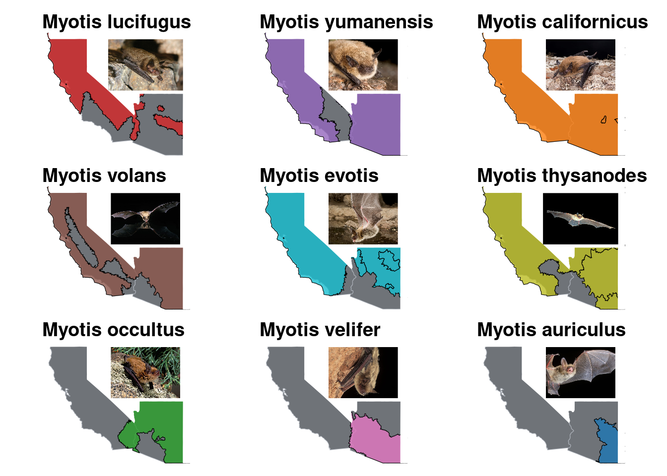
sessionInfo()R version 4.3.1 (2023-06-16)
Platform: x86_64-pc-linux-gnu (64-bit)
Running under: Ubuntu 22.04.3 LTS
Matrix products: default
BLAS: /usr/lib/x86_64-linux-gnu/blas/libblas.so.3.10.0
LAPACK: /usr/lib/x86_64-linux-gnu/lapack/liblapack.so.3.10.0
locale:
[1] LC_CTYPE=C.UTF-8 LC_NUMERIC=C LC_TIME=C.UTF-8
[4] LC_COLLATE=C.UTF-8 LC_MONETARY=C.UTF-8 LC_MESSAGES=C.UTF-8
[7] LC_PAPER=C.UTF-8 LC_NAME=C LC_ADDRESS=C
[10] LC_TELEPHONE=C LC_MEASUREMENT=C.UTF-8 LC_IDENTIFICATION=C
time zone: America/Los_Angeles
tzcode source: system (glibc)
attached base packages:
[1] stats graphics grDevices utils datasets methods base
other attached packages:
[1] patchwork_1.1.3 magick_2.8.1 ggspatial_1.1.9
[4] rnaturalearthdata_0.1.0 rnaturalearth_0.3.4 maps_3.4.1
[7] sf_1.0-14 lubridate_1.9.2 forcats_1.0.0
[10] stringr_1.5.0 dplyr_1.1.3 purrr_1.0.2
[13] readr_2.1.4 tidyr_1.3.0 tibble_3.2.1
[16] ggplot2_3.4.3 tidyverse_2.0.0
loaded via a namespace (and not attached):
[1] tidyselect_1.2.0 farver_2.1.1 fastmap_1.1.1 promises_1.2.1
[5] digest_0.6.33 timechange_0.2.0 lifecycle_1.0.3 magrittr_2.0.3
[9] compiler_4.3.1 rlang_1.1.1 sass_0.4.7 tools_4.3.1
[13] utf8_1.2.3 yaml_2.3.7 knitr_1.44 ggsignif_0.6.4
[17] labeling_0.4.3 curl_5.0.2 bit_4.0.5 sp_2.1-1
[21] classInt_0.4-10 abind_1.4-5 KernSmooth_2.23-22 workflowr_1.7.1
[25] withr_2.5.0 grid_4.3.1 fansi_1.0.5 ggpubr_0.6.0
[29] git2r_0.32.0 e1071_1.7-13 colorspace_2.1-0 scales_1.2.1
[33] cli_3.6.1 rmarkdown_2.25 crayon_1.5.2 generics_0.1.3
[37] rstudioapi_0.15.0 httr_1.4.7 tzdb_0.4.0 DBI_1.1.3
[41] cachem_1.0.8 proxy_0.4-27 parallel_4.3.1 s2_1.1.4
[45] vctrs_0.6.3 jsonlite_1.8.7 carData_3.0-5 car_3.1-2
[49] hms_1.1.3 bit64_4.0.5 ggrepel_0.9.4 rstatix_0.7.2
[53] jquerylib_0.1.4 units_0.8-4 glue_1.6.2 stringi_1.7.12
[57] gtable_0.3.4 later_1.3.1 munsell_0.5.0 pillar_1.9.0
[61] htmltools_0.5.6 R6_2.5.1 wk_0.9.0 rprojroot_2.0.3
[65] vroom_1.6.3 evaluate_0.21 lattice_0.21-8 backports_1.4.1
[69] broom_1.0.5 ggsci_3.0.0 httpuv_1.6.11 bslib_0.5.1
[73] class_7.3-22 Rcpp_1.0.11 xfun_0.40 fs_1.6.3
[77] pkgconfig_2.0.3