creating_merged

Last updated: 2019-10-07

Checks: 4 3

Knit directory: lipids_mvp/

This reproducible R Markdown analysis was created with workflowr (version 1.4.0). The Checks tab describes the reproducibility checks that were applied when the results were created. The Past versions tab lists the development history.

R Markdown file: uncommitted changes

The R Markdown file has unstaged changes. To know which version of the R Markdown file created these results, you’ll want to first commit it to the Git repo. If you’re still working on the analysis, you can ignore this warning. When you’re finished, you can run wflow_publish to commit the R Markdown file and build the HTML.

Environment: empty

Great job! The global environment was empty. Objects defined in the global environment can affect the analysis in your R Markdown file in unknown ways. For reproduciblity it’s best to always run the code in an empty environment.

Seed: set.seed(20190925)

The command set.seed(20190925) was run prior to running the code in the R Markdown file. Setting a seed ensures that any results that rely on randomness, e.g. subsampling or permutations, are reproducible.

Session information: recorded

Great job! Recording the operating system, R version, and package versions is critical for reproducibility.

Cache: detected

The following chunks had caches available:

create table
session-info-chunk-inserted-by-workflowr
unnamed-chunk-1
unnamed-chunk-2
unnamed-chunk-3
unnamed-chunk-4
unnamed-chunk-5
unnamed-chunk-6
unnamed-chunk-7

To ensure reproducibility of the results, delete the cache directory workingwithdata_cache and re-run the analysis. To have workflowr automatically delete the cache directory prior to building the file, set delete_cache = TRUE when running wflow_build() or wflow_publish().

File paths: absolute

Using absolute paths to the files within your workflowr project makes it difficult for you and others to run your code on a different machine. Change the absolute path(s) below to the suggested relative path(s) to make your code more reproducible.

absolute	relative
~/lipids_mvp/data/merged_z.txt	data/merged_z.txt
~/lipids_mvp/data/znew.txt	data/znew.txt
~/lipids_mvp/data/max_ld_block.txt	data/max_ld_block.txt
~/lipids_mvp/data/EDcov.Rds	data/EDcov.Rds
~/lipids_mvp/data/mashresult.rds	data/mashresult.rds
~/lipids_mvp/data/mashcomplete.rds	data/mashcomplete.rds
~/lipids_mvp/data/ash.rds	data/ash.rds
~/lipids_mvp/data/merged_p.txt	data/merged_p.txt

Repository version: d8023e7

Great! You are using Git for version control. Tracking code development and connecting the code version to the results is critical for reproducibility. The version displayed above was the version of the Git repository at the time these results were generated.

Note that you need to be careful to ensure that all relevant files for the analysis have been committed to Git prior to generating the results (you can use wflow_publish or wflow_git_commit). workflowr only checks the R Markdown file, but you know if there are other scripts or data files that it depends on. Below is the status of the Git repository when the results were generated:


Ignored files:
    Ignored:    .DS_Store
    Ignored:    .Rhistory
    Ignored:    analysis/.DS_Store
    Ignored:    analysis/.RData
    Ignored:    analysis/.Rhistory
    Ignored:    analysis/looking_at_significance_cache/
    Ignored:    analysis/workingwithdata_cache/
    Ignored:    data/.DS_Store
    Ignored:    data/Archive.zip.gz
    Ignored:    data/EDcov.Rds
    Ignored:    data/ash.rds
    Ignored:    data/gtexcolors.txt
    Ignored:    data/mashcomplete.rds
    Ignored:    data/mashcomplete.rds.zip
    Ignored:    data/max_ld_block.txt
    Ignored:    data/merged_betas.txt
    Ignored:    data/merged_p.txt
    Ignored:    data/merged_se.txt
    Ignored:    data/merged_z.txt
    Ignored:    data/znew.txt
    Ignored:    docs/.DS_Store

Unstaged changes:
    Modified:   analysis/workingwithdata.Rmd

Note that any generated files, e.g. HTML, png, CSS, etc., are not included in this status report because it is ok for generated content to have uncommitted changes.

These are the previous versions of the R Markdown and HTML files. If you’ve configured a remote Git repository (see ?wflow_git_remote), click on the hyperlinks in the table below to view them.

File	Version	Author	Date	Message
Rmd	079589b	Sarah Urbut	2019-10-07	Update
html	079589b	Sarah Urbut	2019-10-07	Update
Rmd	7142cc6	Sarah Urbut	2019-10-04	Updated plots
html	7142cc6	Sarah Urbut	2019-10-04	Updated plots
Rmd	73da9ad	Sarah Urbut	2019-10-03	Update
html	73da9ad	Sarah Urbut	2019-10-03	Update
html	ca158bf	Sarah Urbut	2019-10-03	Update docs

R Markdown

Here we will try to merge based on common chr.position (per Hg18) names.

We recognize that the alleles have been flipped to make all effects positive Let’s use HDL as reference

ref=m[,3]

for(x in seq(1:3)){
  betaindex=4+2*x
  beta=m[,betaindex]
  allele=betaindex-1
  a=m[,allele]
  test=a==ref;test[test=="FALSE"]=-1
  beta=beta*test
  m[,betaindex]=beta}

head(m)
write.table(m,"merged_betas.txt")

## Creating SE Table
n=merge(hdl[,c(1,3,7)],ldl[,c(1,7)],by=1);names(n)[3]="hdl";names(n)[4]="ldl"
n=merge(n,tg[,c(1,7)],by=1);names(n)[5]="tg"
n=merge(n,tc[,c(1,7)],by=1);names(n)[6]="tc"
write.table(n,"merged_se.txt")

z=m[,c(4,6,8,10)]/n[,c(3:6)]
z=cbind(m[,c(1,2)],z)
write.table(z,"merged_z.txt")

To run mashr, we need a matrix of maxes. The best way to do this is to choose the max effect across conditions per LD block, as described in Pickrell et al. Only then can we assume the maxes used to create covariance matrices are truly linearly independent. We will select SNPS falling within each of the 1700 LD blocks and choose SNP with maximum absolute effect acrtoss conditions.

#z=read.table("~/lipids_mvp/data/merged_z.txt")
# 
# bed=read.table("~/Downloads/ld_chunk.bed")
# head(bed)
# z=z[1:2437099,]### last 3 are rsIDs from mislabeled columns
# library("reshape")
# df=transform(z, foo = colsplit(z$SNP_hg18, split = "\\:", names = c('Chr', 'Pos')))
# 
# znew=cbind(df$foo.Chr,df$foo.Pos,z[,-1])
# maxes=apply(znew[,c("hdl","ldl","tg","tc")],1,function(x){max(abs(x))})
# znew=cbind(znew,maxes)

max_block=data.frame(matrix(ncol = ncol(znew), nrow = nrow(bed)))
colnames(max_block)=colnames(znew)
for(i in 1:nrow(bed)){
  chr=bed[i,1]
  start=bed[i,2]
  stop=bed[i,3]
  in_chrom=znew[znew$`df$foo.Chr`==chr,]
  goodguys=in_chrom[in_chrom$`df$foo.Pos`>start&in_chrom$`df$foo.Pos`<stop,]
 if(nrow(goodguys)>0) {
    z.max=which.max(goodguys[,"maxes"])
    z_good=goodguys[z.max,]
    } else {
      z_good=rep(0,ncol(max_block))
    }
  z_good=data.table(z_good,stringsAsFactors = T)
  z_good$`df$foo.Chr`=as.character(z_good$`df$foo.Chr`)
  z_good$rsid=as.character(z_good$rsid)
  max_block[i,]=z_good
  #print(i)
}

max_block=na.omit(max_block)
write.table(max_block,"max_ld_block.txt")

Now, we’re ready to mash!

znew=read.table("~/lipids_mvp/data/znew.txt")
library("mashr")
library("flashr")
max_block=read.table("~/lipids_mvp/data/max_ld_block.txt")
source('~/Dropbox/jointData/flashscript.R')
# identify a random subset of 20000 tests
random.subset = sample(1:nrow(znew),20000)
zmash=as.matrix(znew[,c("hdl","ldl","tg","tc")]);rownames(zmash)=znew$rsid
data.temp = mash_set_data(zmash[random.subset,],alpha = 1)
Vhat = estimate_null_correlation_simple(data.temp)
library("lattice")
clrs = colorRampPalette((c("#D73027","#FC8D59","#FEE090","#FFFFBF", "#E0F3F8","#91BFDB","#4575B4")))(64)

print(levelplot(Vhat,col.regions = clrs,xlab = "",ylab = "",colorkey = TRUE,main="VHAT"))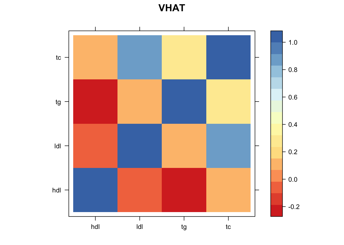

Version	Author	Date
ca158bf	Sarah Urbut	2019-10-03

rm(data.temp)
data.random = mash_set_data(zmash[random.subset,],alpha = 1,V=Vhat)

zmax=apply(max_block[,c(4:7)],2,function(x){as.numeric(x)});rownames(zmax)=max_block$rsid
data.strong = mash_set_data(zmax,alpha = 1,V=Vhat)

U.pca = cov_pca(data.strong,3)

# U.flash=cov_flash(data.strong, non_canonical = TRUE)
# X.center = apply(data.strong$Bhat, 2, function(x) x - mean(x))
# U.ed = cov_ed(data.strong, c(U.flash, U.pca, list("XX" = t(X.center) %*% X.center / nrow(X.center))))
# saveRDS(U.ed,"~/lipids_mvp/data/EDcov.Rds")

U.ed=readRDS("~/lipids_mvp/data/EDcov.Rds")
U.c = cov_canonical(data.random)
m = mash(data.random, Ulist = c(U.ed,U.c),outputlevel = 1)

 - Computing 20000 x 321 likelihood matrix.
 - Likelihood calculations took 2.13 seconds.
 - Fitting model with 321 mixture components.
 - Model fitting took 31.55 seconds.

k=length(m$fitted_g$Ulist)
l=length(m$fitted_g$grid)
pimat=matrix(m$fitted_g$pi[-1],nrow=l,byrow=T)
colnames(pimat)=names(m$fitted_g$pi)[2:(k+1)]
barplot(colSums(pimat),las=2)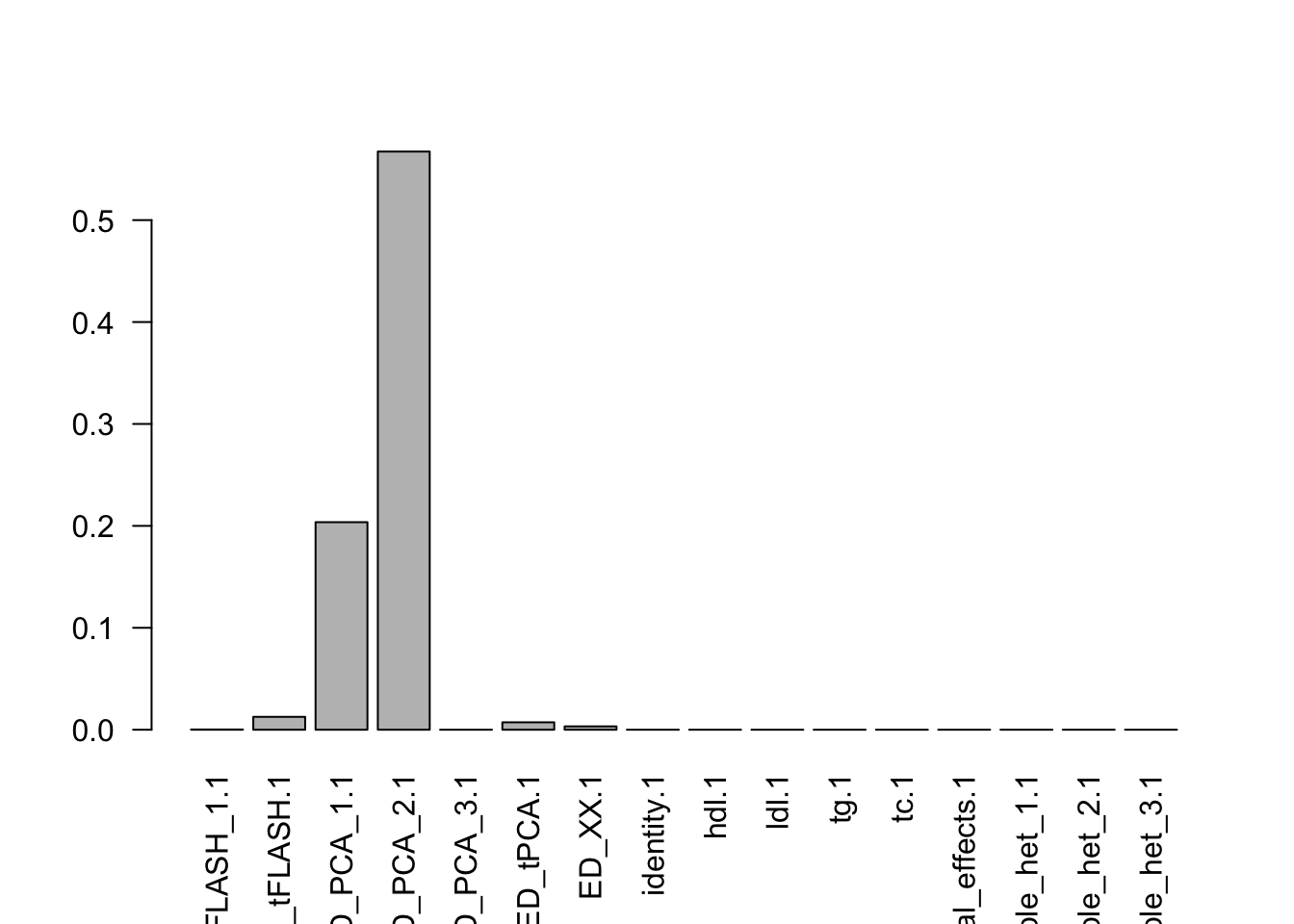

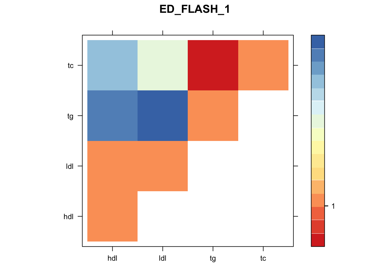
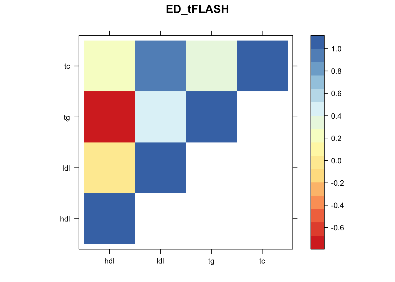
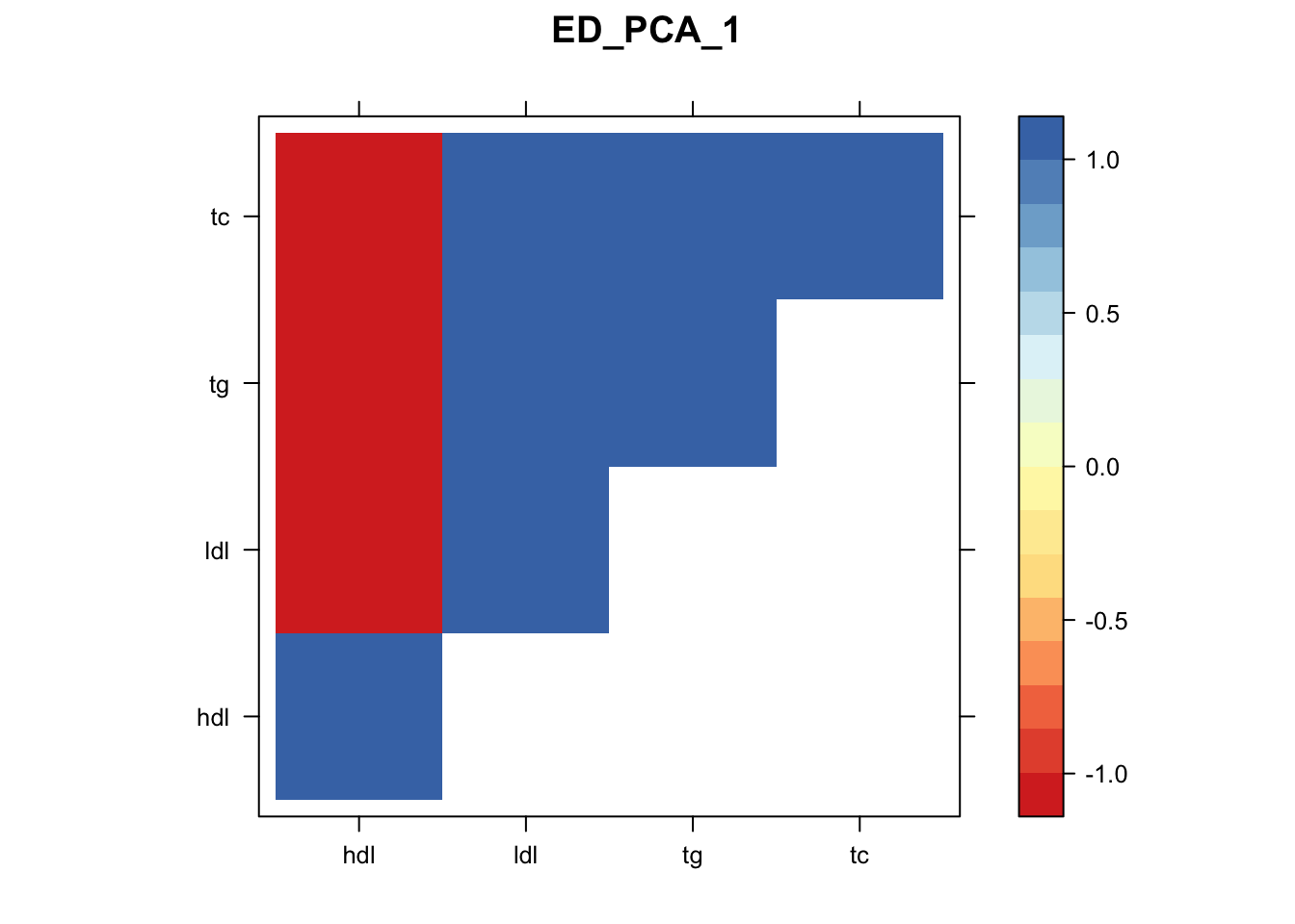
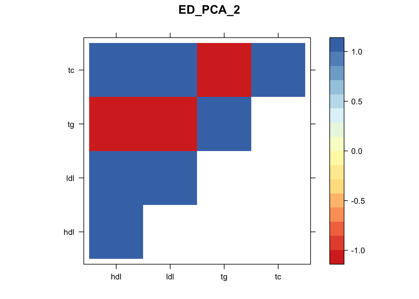
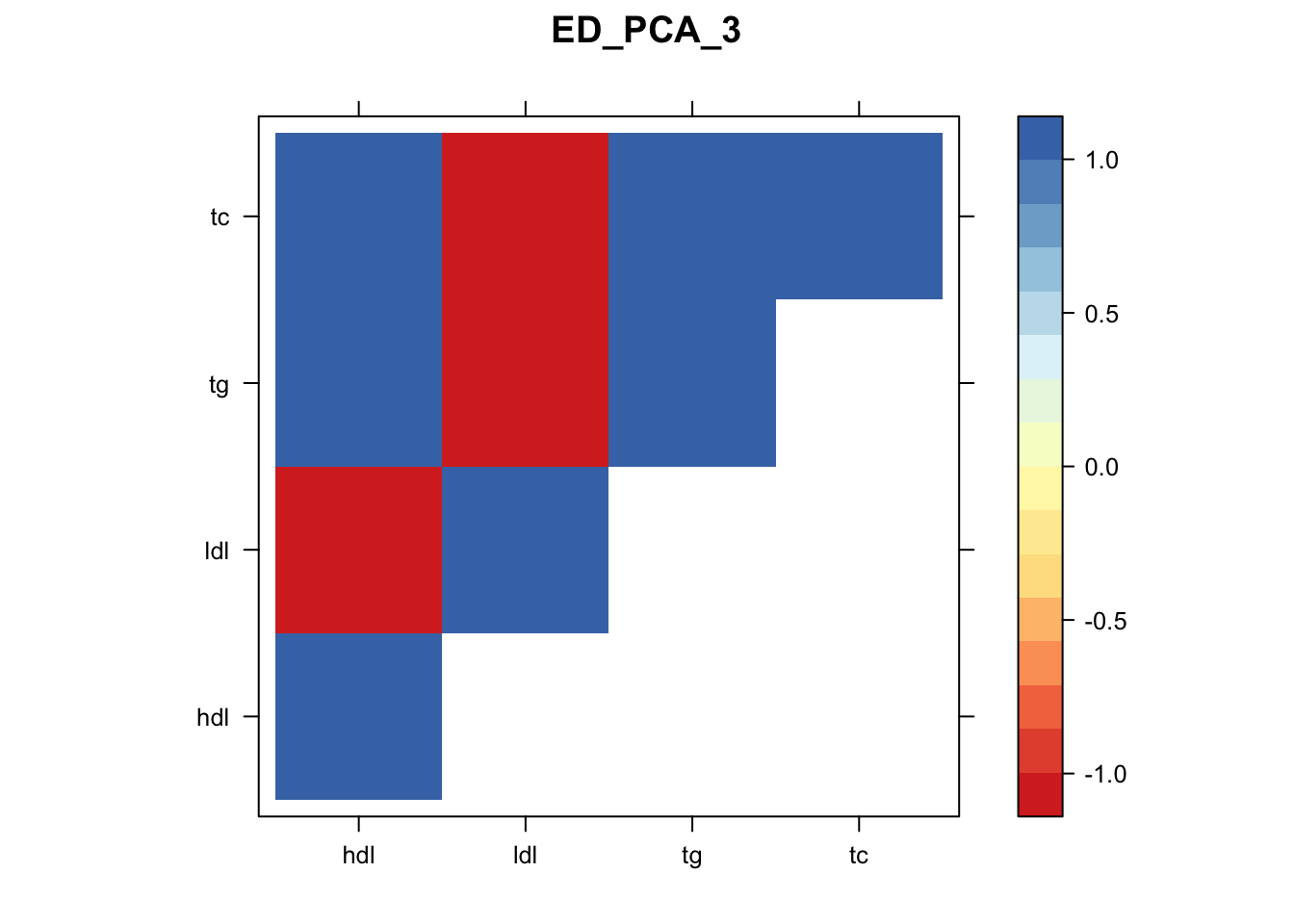
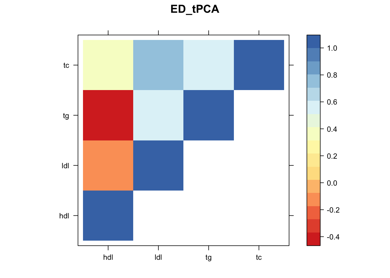
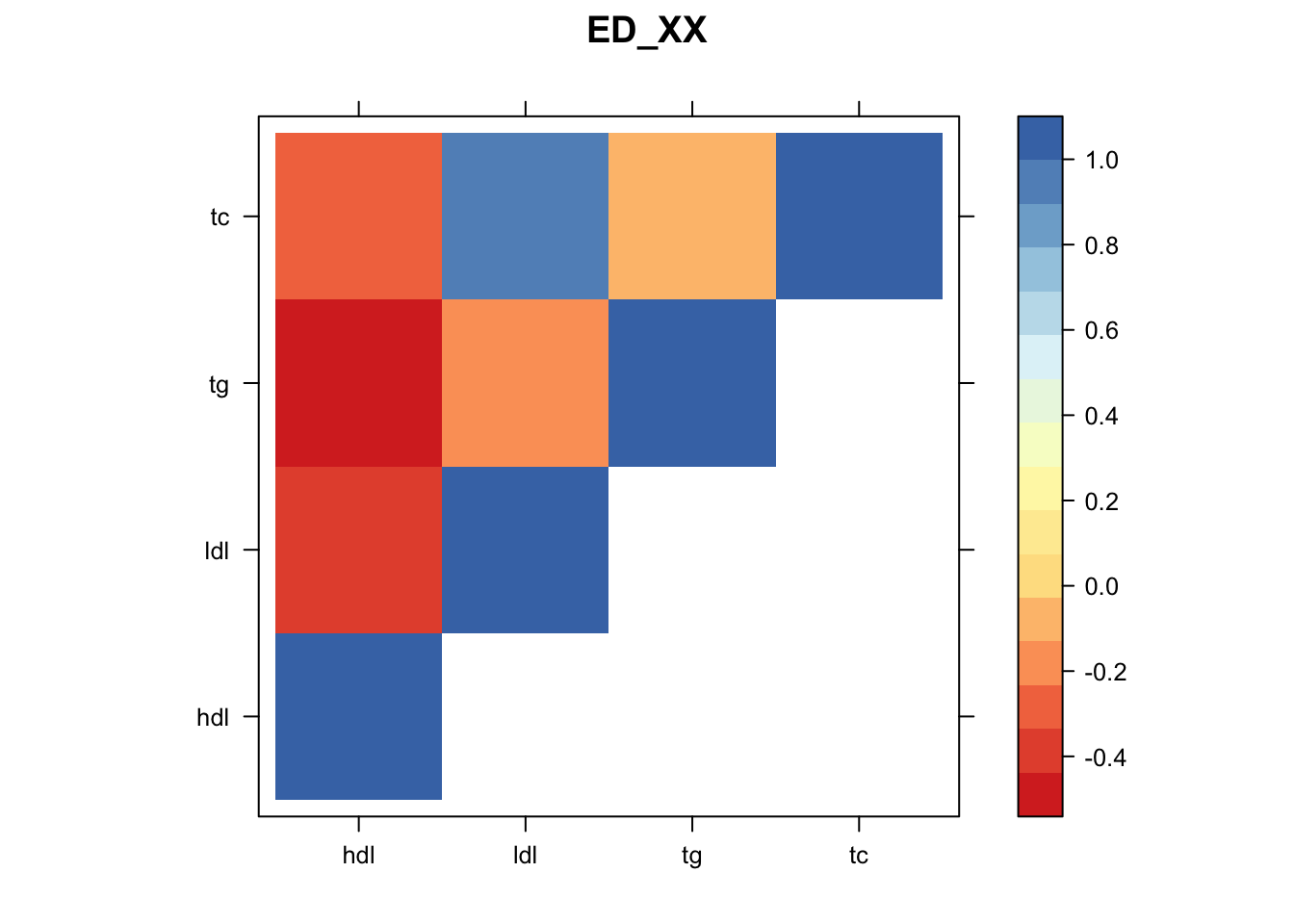
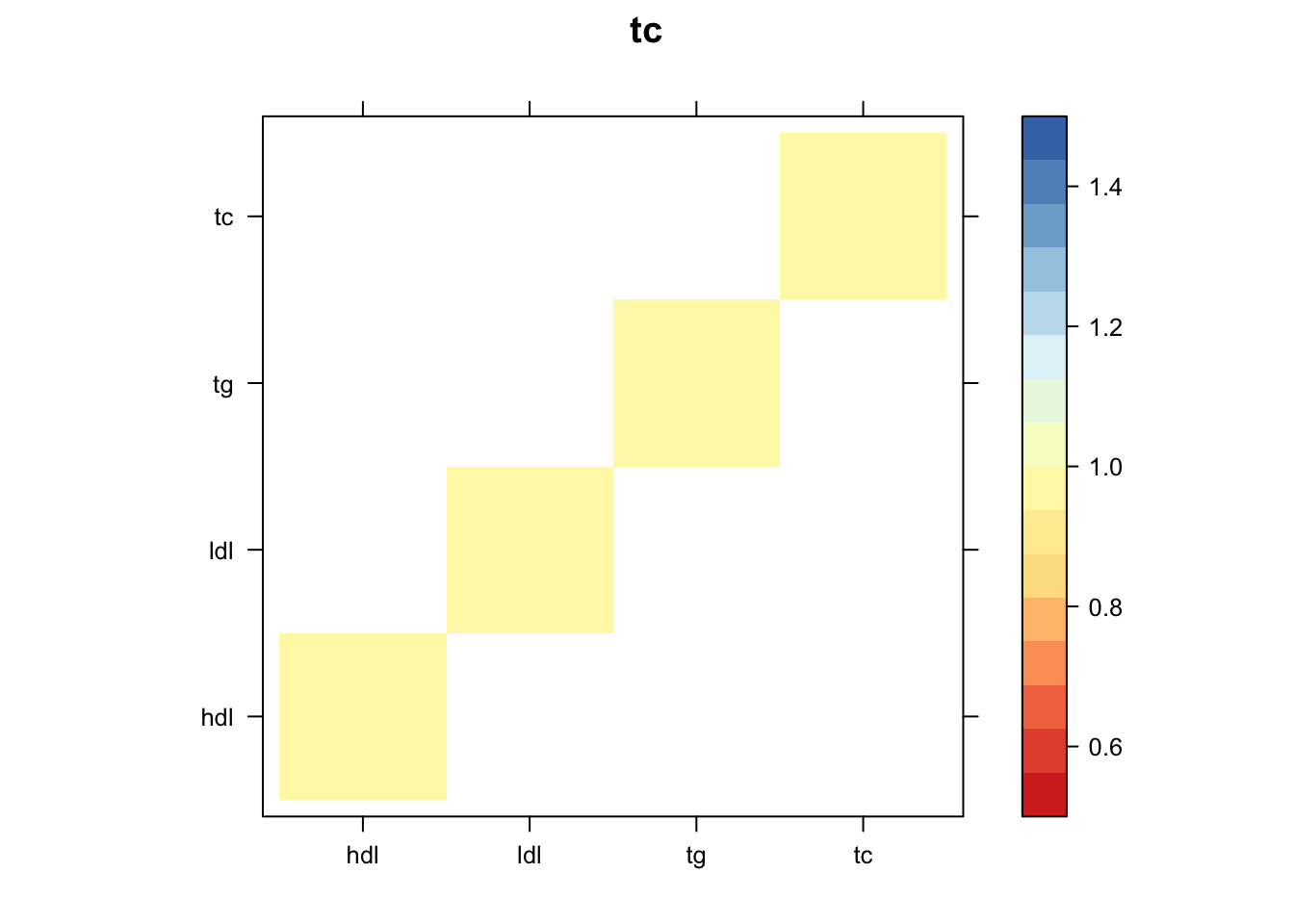
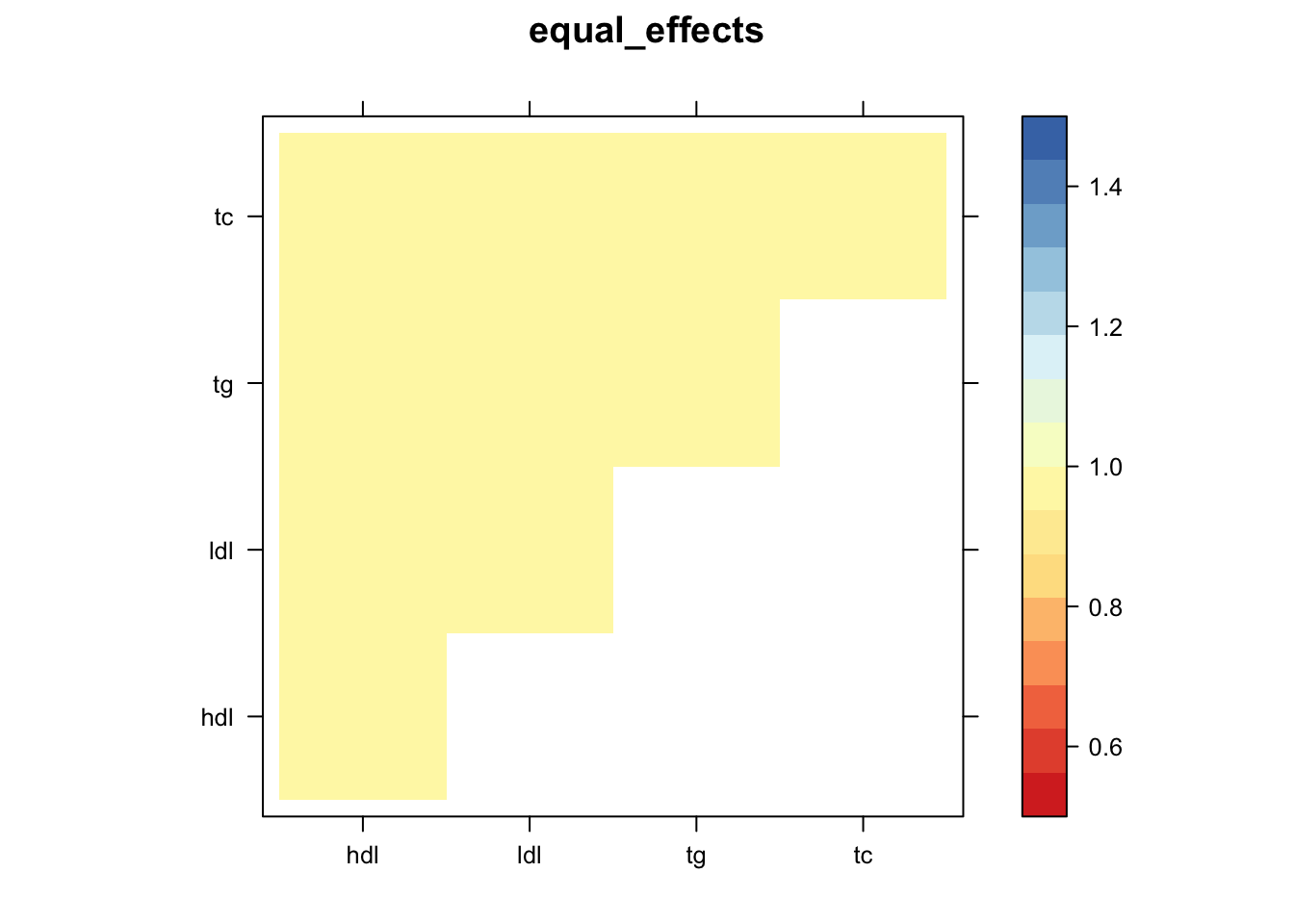
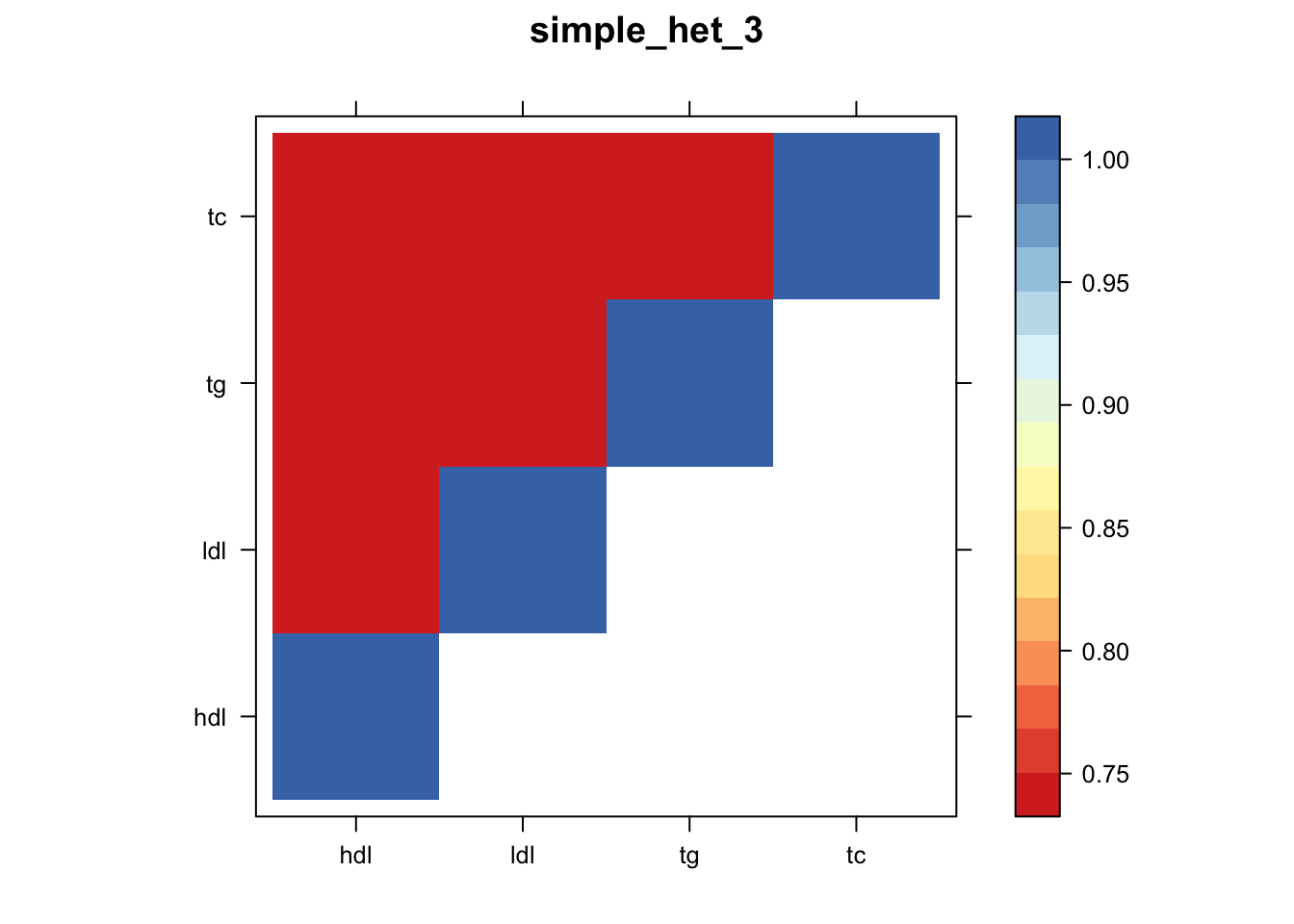
Now, let’s plot the patterns of sharing as the correlation matrix of the estimated covariance matrices. We can see that from the barplot, there are the following matrices: ED_FLASH_1.1, ED_tFLASH.1, ED_PCA_1.1, ED_PCA_2.1, ED_PCA_3.1, ED_tPCA.1, ED_XX.1, identity.1, hdl.1, ldl.1, tg.1, tc.1, equal_effects.1, simple_het_1.1, simple_het_2.1, simple_het_3.1.

library("lattice")
for(i in 1:k){
  z.num=as.matrix(cov2cor(m$fitted_g$Ulist[[i]]))
  colnames(z.num)=row.names(z.num)=colnames(zmash)
clrs = colorRampPalette((c("#D73027","#FC8D59","#FEE090","#FFFFBF", "#E0F3F8","#91BFDB","#4575B4")))(64)
z.num[lower.tri(z.num)] = NA
print(levelplot(z.num,col.regions = clrs,xlab = "",ylab = "",colorkey = TRUE,main=paste0(names(m$fitted_g$Ulist)[[i]])))
}

Version	Author	Date
ca158bf	Sarah Urbut	2019-10-03

Version	Author	Date
ca158bf	Sarah Urbut	2019-10-03

Version	Author	Date
ca158bf	Sarah Urbut	2019-10-03

Version	Author	Date
ca158bf	Sarah Urbut	2019-10-03

Version	Author	Date
ca158bf	Sarah Urbut	2019-10-03

Version	Author	Date
ca158bf	Sarah Urbut	2019-10-03

Version	Author	Date
ca158bf	Sarah Urbut	2019-10-03

Warning in cov2cor(m$fitted_g$Ulist[[i]]): diag(.) had 0 or NA entries;
non-finite result is doubtful

Version	Author	Date
ca158bf	Sarah Urbut	2019-10-03

Warning in cov2cor(m$fitted_g$Ulist[[i]]): diag(.) had 0 or NA entries;
non-finite result is doubtful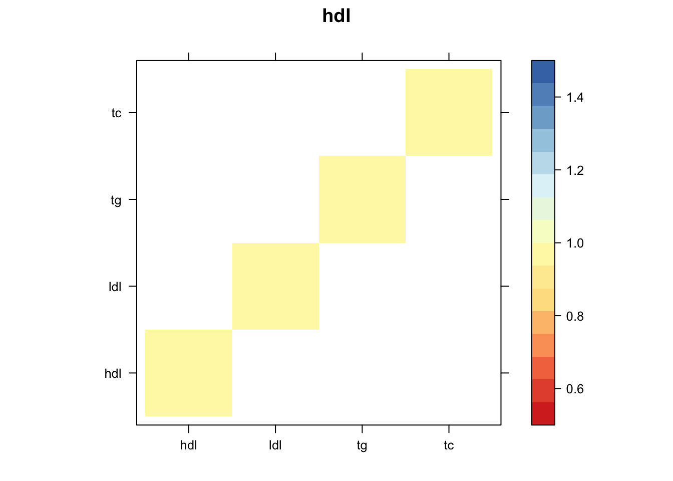

Version	Author	Date
ca158bf	Sarah Urbut	2019-10-03

Warning in cov2cor(m$fitted_g$Ulist[[i]]): diag(.) had 0 or NA entries;
non-finite result is doubtful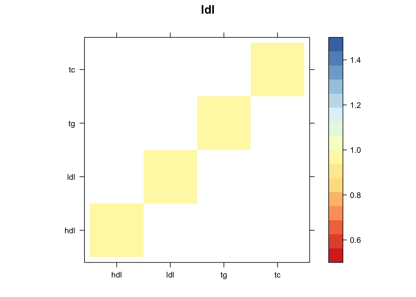

Version	Author	Date
ca158bf	Sarah Urbut	2019-10-03

Warning in cov2cor(m$fitted_g$Ulist[[i]]): diag(.) had 0 or NA entries;
non-finite result is doubtful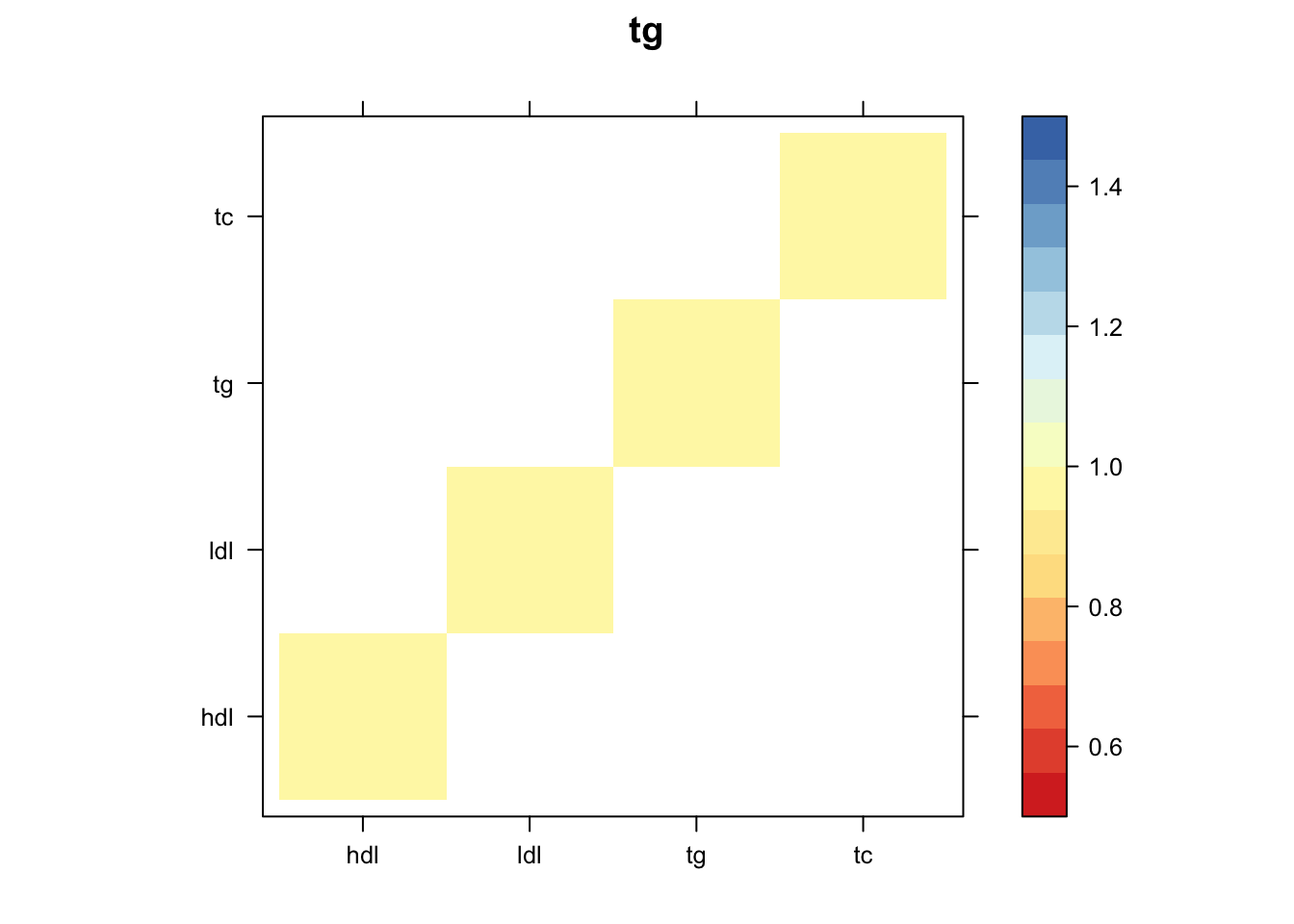

Version	Author	Date
ca158bf	Sarah Urbut	2019-10-03

Version	Author	Date
ca158bf	Sarah Urbut	2019-10-03

Version	Author	Date
ca158bf	Sarah Urbut	2019-10-03

Version	Author	Date
ca158bf	Sarah Urbut	2019-10-03

Version	Author	Date
ca158bf	Sarah Urbut	2019-10-03

Version	Author	Date
ca158bf	Sarah Urbut	2019-10-03

Now we can compute posteriors,

mash.data=mash_set_data(zmash,V = Vhat,alpha = 1)

m$result=mash_compute_posterior_matrices(m, mash.data, algorithm.version = "Rcpp")
saveRDS(m,"~/lipids_mvp/data/mashresult.rds")

Let’s take a look:

m=readRDS("~/lipids_mvp/data/mashcomplete.rds")
head(m$result$PosteriorMean)

                   hdl         ldl           tg          tc
rs1172982   0.06015013  0.10542699  0.002012870  0.11805417
rs1172981   0.28626776  0.05244131 -0.188875181  0.10104744
rs11166327 -0.11849671 -0.01776064  0.085266561 -0.03603278
rs4908018   0.31317283  0.05412064 -0.209288205  0.10681010
rs2392072   0.05437422  0.09588751  0.002789049  0.10754994
rs12129588  0.34618757  0.07306129 -0.225178675  0.13174043

head(m$result$lfsr)

                 hdl       ldl        tg        tc
rs1172982  0.6283334 0.5228317 0.6311741 0.5223916
rs1172981  0.4205101 0.4270629 0.4196412 0.4274541
rs11166327 0.5462653 0.5541580 0.5434676 0.5553625
rs4908018  0.4001065 0.4115782 0.3989821 0.4121384
rs2392072  0.6310612 0.5339740 0.6339992 0.5334568
rs12129588 0.3834876 0.3805365 0.3827029 0.3809647

lfsr=m$result$lfsr
s=rowSums(lfsr<=0.05)

hist(s[s>1],freq=FALSE,main="Number of Conditions")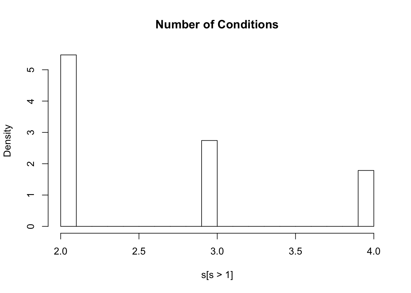

#ash.z=apply(zmash,2,function(x){ashr::ash(x,sebetahat = rep(1,length(x)))})
#saveRDS(ash.z,"../data/ash.rds")
ash.z=readRDS("~/lipids_mvp/data/ash.rds")
ashresults=cbind(ash.z$hdl$result$PosteriorMean,ash.z$ldl$result$PosteriorMean,ash.z$tg$result$PosteriorMean,ash.z$tc$result$PosteriorMean)
ashlfsr=cbind(ash.z$hdl$result$lfsr,ash.z$ldl$result$lfsr,ash.z$tg$result$lfsr,ash.z$tc$result$lfsr)

sum(ashlfsr<0.05)

[1] 29301

Here 29301 SNPS x Conditions are less than 0.05 using a univariate appropach and 80539 are less than 0.05 with a joint approach, a roughly 250% increase. Furthermore, 32176 SNPS are significant in at least one condition wiht a juint approach, while 18099 with a univariate one.

p=read.table("~/lipids_mvp/data/merged_p.txt")
library(knitr)
library(kableExtra)
dt <- cbind(c(paste("Bonferroni=",sum(p<=5e-8)),paste("univariate_ash=",sum(ashlfsr<0.05)),paste("mv_mash=",sum(lfsr<0.05))))

dt <- cbind(c(sum(p<=5e-8),sum(ashlfsr<0.05),sum(lfsr<0.05)))
dt=cbind(dt,c(sum(rowSums(p<=5e-8)>0),sum(rowSums(ashlfsr<0.05)>0),sum(rowSums(lfsr<0.05)>0)))
rownames(dt)=c("Bonferroni","UnivariateAsh","Mash")
colnames(dt)=c("Overall All Associations","Per Snp, in at least one")           
              
kable(dt)

	Overall All Associations	Per Snp, in at least one
Bonferroni	14005	8595
UnivariateAsh	29301	18099
Mash	80539	32176

dt %>%
  kable() %>%
  kable_styling()

	Overall All Associations	Per Snp, in at least one
Bonferroni	14005	8595
UnivariateAsh	29301	18099
Mash	80539	32176

sessionInfo()

R version 3.5.2 (2018-12-20)
Platform: x86_64-apple-darwin15.6.0 (64-bit)
Running under: macOS Mojave 10.14.6

Matrix products: default
BLAS: /Library/Frameworks/R.framework/Versions/3.5/Resources/lib/libRblas.0.dylib
LAPACK: /Library/Frameworks/R.framework/Versions/3.5/Resources/lib/libRlapack.dylib

locale:
[1] en_US.UTF-8/en_US.UTF-8/en_US.UTF-8/C/en_US.UTF-8/en_US.UTF-8

attached base packages:
[1] stats     graphics  grDevices utils     datasets  methods   base     

other attached packages:
[1] lattice_0.20-38   flashr_0.6-3      mashr_0.2.21.0631 ashr_2.2-37      
[5] reshape_0.8.8    

loaded via a namespace (and not attached):
 [1] Rcpp_1.0.1        pillar_1.4.2      compiler_3.5.2   
 [4] git2r_0.26.1      plyr_1.8.4        highr_0.8        
 [7] workflowr_1.4.0   iterators_1.0.10  tools_3.5.2      
[10] digest_0.6.20     tibble_2.1.3      gtable_0.3.0     
[13] evaluate_0.14     pkgconfig_2.0.2   rlang_0.4.0      
[16] Matrix_1.2-17     foreach_1.4.4     rstudioapi_0.10  
[19] yaml_2.2.0        parallel_3.5.2    mvtnorm_1.0-11   
[22] xfun_0.8          dplyr_0.8.3       stringr_1.4.0    
[25] knitr_1.23        fs_1.3.1          tidyselect_0.2.5 
[28] rprojroot_1.3-2   grid_3.5.2        glue_1.3.1       
[31] R6_2.4.0          rmarkdown_1.14    mixsqp_0.1-97    
[34] rmeta_3.0         reshape2_1.4.3    purrr_0.3.2      
[37] ggplot2_3.2.0     magrittr_1.5      scales_1.0.0     
[40] backports_1.1.4   codetools_0.2-16  htmltools_0.3.6  
[43] MASS_7.3-51.4     abind_1.4-5       assertthat_0.2.1 
[46] softImpute_1.4    colorspace_1.4-1  stringi_1.4.3    
[49] lazyeval_0.2.2    munsell_0.5.0     doParallel_1.0.14
[52] pscl_1.5.2        truncnorm_1.0-8   SQUAREM_2017.10-1
[55] crayon_1.3.4

creating_merged_lipids

R Markdown