Spatially resticted genes

workflowr

• Summary
• Checks
• Past versions

Last updated: 2024-11-01

Checks: 7 0

Knit directory: spatialsnippets/

This reproducible R Markdown analysis was created with workflowr (version 1.7.1). The Checks tab describes the reproducibility checks that were applied when the results were created. The Past versions tab lists the development history.

---

R Markdown file: up-to-date

Great! Since the R Markdown file has been committed to the Git repository, you know the exact version of the code that produced these results.

Environment: empty

Great job! The global environment was empty. Objects defined in the global environment can affect the analysis in your R Markdown file in unknown ways. For reproduciblity it’s best to always run the code in an empty environment.

Seed: set.seed(20231017)

The command set.seed(20231017) was run prior to running the code in the R Markdown file. Setting a seed ensures that any results that rely on randomness, e.g. subsampling or permutations, are reproducible.

Session information: recorded

Great job! Recording the operating system, R version, and package versions is critical for reproducibility.

Cache: none

Nice! There were no cached chunks for this analysis, so you can be confident that you successfully produced the results during this run.

File paths: relative

Great job! Using relative paths to the files within your workflowr project makes it easier to run your code on other machines.

Repository version: 6cf65ff

Great! You are using Git for version control. Tracking code development and connecting the code version to the results is critical for reproducibility.

The results in this page were generated with repository version 6cf65ff. See the Past versions tab to see a history of the changes made to the R Markdown and HTML files.

Note that you need to be careful to ensure that all relevant files for the analysis have been committed to Git prior to generating the results (you can use wflow_publish or wflow_git_commit). workflowr only checks the R Markdown file, but you know if there are other scripts or data files that it depends on. Below is the status of the Git repository when the results were generated:

Ignored files:
    Ignored:    .Rhistory
    Ignored:    .Rproj.user/
    Ignored:    analysis/contributions.nb.html
    Ignored:    analysis/e_neighbourcellchanges.nb.html
    Ignored:    analysis/e_spatiallyRestrictedGenesVoyager.nb.html
    Ignored:    analysis/figure/
    Ignored:    analysis/g_toolkits.nb.html
    Ignored:    analysis/glossary.nb.html
    Ignored:    renv/library/
    Ignored:    renv/staging/

Untracked files:
    Untracked:  code/scwat-at_betweenClusters_heterotypic_score_functions.R
    Untracked:  other/

Note that any generated files, e.g. HTML, png, CSS, etc., are not included in this status report because it is ok for generated content to have uncommitted changes.

---

These are the previous versions of the repository in which changes were made to the R Markdown (analysis/e_spatiallyRestrictedGenes.Rmd) and HTML (docs/e_spatiallyRestrictedGenes.html) files. If you’ve configured a remote Git repository (see ?wflow_git_remote), click on the hyperlinks in the table below to view the files as they were in that past version.

File	Version	Author	Date	Message
Rmd	6cf65ff	swbioinf	2024-11-01	wflow_publish("analysis/e_spatiallyRestrictedGenes.Rmd")
Rmd	45cde50	swbioinf	2024-10-28	adding halfbuilt files
html	4e21b4e	swbioinf	2024-07-03	Build site.
Rmd	a10809a	swbioinf	2024-07-03	wflow_publish("analysis/e_spatiallyRestrictedGenes.Rmd")
Rmd	fd64e30	swbioinf	2024-06-18	new plots

---

Overview

It is possible to test for genes that are expressed in a spatially non-random pattern. These might be restricted to regions of a tissu (e.g. epithelia), with a very punctate expression in selected cells only (e.g. immunoglobulins in plasma cells).

One popular approach to find these genes is the MoransI test of spatial autocorrelation.

This example will show how to use the morans test within seurat to find spatially restricted genes.

This requires:

• X,Y coordinates of individual transcripts, or their cells.

There is no need for celltype annotation.

For example:

• What cells are sptially restricted in this tissue, are they in a layer of epithelial or elsewhere.

Steps:

1. Breif description of steps involved in test
2. If appropriate.

Worked example

Paper Microglia-astrocyte crosstalk in the amyloid plaque niche of an Alzheimer’s disease mouse model, as revealed by spatial transcriptomics (mallachMicrogliaastrocyteCrosstalkAmyloid2024?) explores the spatial transcritome of amaloid plaques in a mouse model.

Their work includes an analysis of cosMX samples from of 4 mouse brain samples.

This example will test which genes are expressed in a spatially restricted pattern; e.g. along the boarder of a feature, in clumps or in some way non-random. This will be done for each sample, independently of any celltype annotations.

Load libraries and data

library(Seurat)
library(tidyverse)
library(DT)

# Needed for moransI
#renv::install('Rfast2') # needs GSL installed on system
#renv::install('ape')

dataset_dir      <- '~/projects/spatialsnippets/datasets/GSE263793_Mallach2024_AlzPlaque/processed_data/'
seurat_file_01_preprocessed <- file.path(dataset_dir,  "GSE263793_AlzPlaque_seurat_01_preprocessed.RDS")

so <- readRDS(seurat_file_01_preprocessed)

Spatially variable features

Morans test can be slow to run, so save time by only running it on VariableFeatures (non variable features are unlikely to be spatially restricted anyway!).

For the purpose of this demo, only test the top 10. The actual number for a real experiment could be judged from the variable features plot below, e.g. 100-200 (or more, depending on your panel!).

num_variable_features = 10 # Test only, Would be 100+ in real life
so <-  FindVariableFeatures(so, nfeatures=num_variable_features)
VariableFeaturePlot(so)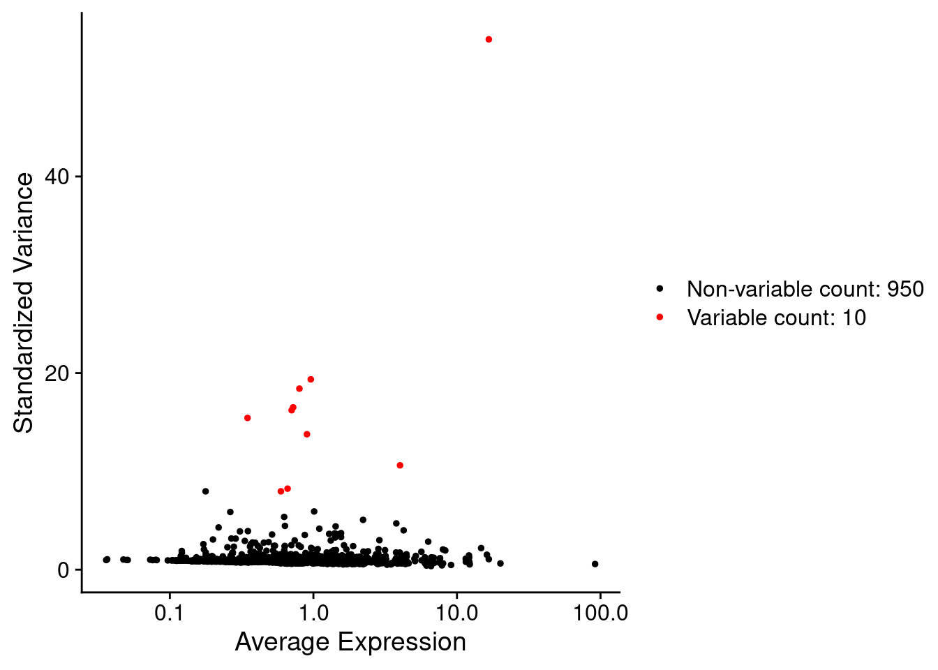

We will look for variable features on each of our slides. X and Y coordinates from each slide are entirely separate. With a larger number of slides, this could be done in a for loop.

so.sample <- subset( so, subset= sample == 'sample1')

Right now, there is a bug with the current FindSpatiallyVariableFeatures function. https://github.com/satijalab/seurat/issues/8226

As a temporary workaround, using a customised version of this that avoids the issue in just this dataset. NB: The edit simply changes the way the data is stored in the metadata: object[[names(x = svf.info)]] <- svf.info

# Workaround 
# Available: https://github.com/swbioinf/spatialsnippets/blob/main/code/spatially_variable_features_code.R
source("code/spatially_variable_features_code.R")
so.sample <- FindSpatiallyVariableFeatures.Seurat_EDITED(
  so.sample, 
  assay = "RNA", 
  features = VariableFeatures(so.sample),    
  selection.method = "moransi",
  layer = "counts")

[1] ">>>> USING EDITED FUNCTION!!!! <<<"

## What it should be:
## Try this command first!
#so.sample <- FindSpatiallyVariableFeatures(
#  so.sample, 
#  assay = "RNA", 
#  features = VariableFeatures(so.sample),    
#  selection.method = "moransi",
#  layer = "counts")

FindSpatiallyVariableFeatures returns a seurat object with the moransI scores embedded in the feature metatdata of the ‘RNA’ assay.

gene_metadata <- so.sample[["RNA"]]@meta.data
#NB: This is a seperate table to the *cell* metadata found at so.sample@meta.data
# so.sample[['RNA']]  retreives the 'RNA' assay.

DT::datatable(head(gene_metadata))

The whole gene-metadata includes other columns, and in fact the columns we are interested in only have values for the ‘variable’ genes that we tested. So, make a summary table with just the relevant data.

gene_metadata_morans <- 
  filter(gene_metadata, !is.na(moransi.spatially.variable.rank)) %>%
  select(feature, 
         MoransI_observed, MoransI_p.value, moransi.spatially.variable,moransi.spatially.variable.rank) %>% 
  arrange(moransi.spatially.variable.rank)
  
head(gene_metadata_morans)

  feature MoransI_observed MoransI_p.value moransi.spatially.variable
1   Ptgds       0.32296951    0.0009756098                       TRUE
2    Penk       0.15905615    0.0009756098                       TRUE
3    Drd4       0.08720462    0.0009756098                       TRUE
4  Lilra5       0.08718934    0.0009756098                       TRUE
5     Vtn       0.05282752    0.0009756098                       TRUE
6   Acta2       0.02569337    0.0009756098                       TRUE
  moransi.spatially.variable.rank
1                               1
2                               2
3                               3
4                               4
5                               5
6                               6

Plot results

We can pull out the most significant genes from that table.

top_genes = gene_metadata_morans$feature[1:3]
top_genes

[1] "Ptgds" "Penk"  "Drd4" 

Here we are plotting the top 3 genes on that slide. Each has a different but clear reasons for being spatially restricted. Ptgds and Penk seem to be restricted to differnet regions of the tissue. Drd4 is a little different; it seems to have high expression in a subset of cells - its proximity to itself also triggers the significance n the morans test.

NB: Genes without any sort of spatial pattern might still have some sort of morans test significance - since they’re still restricted to the tissue itself it isn’t random.

ImageDimPlot(so.sample,  fov = "AD2.AD3.CosMx",
             molecules = top_genes, 
             group.by = 'sample', cols = c("grey30"), # Make all cells grey.
             boundaries = "segmentation",
             border.color = 'black', axes = T, crop=TRUE)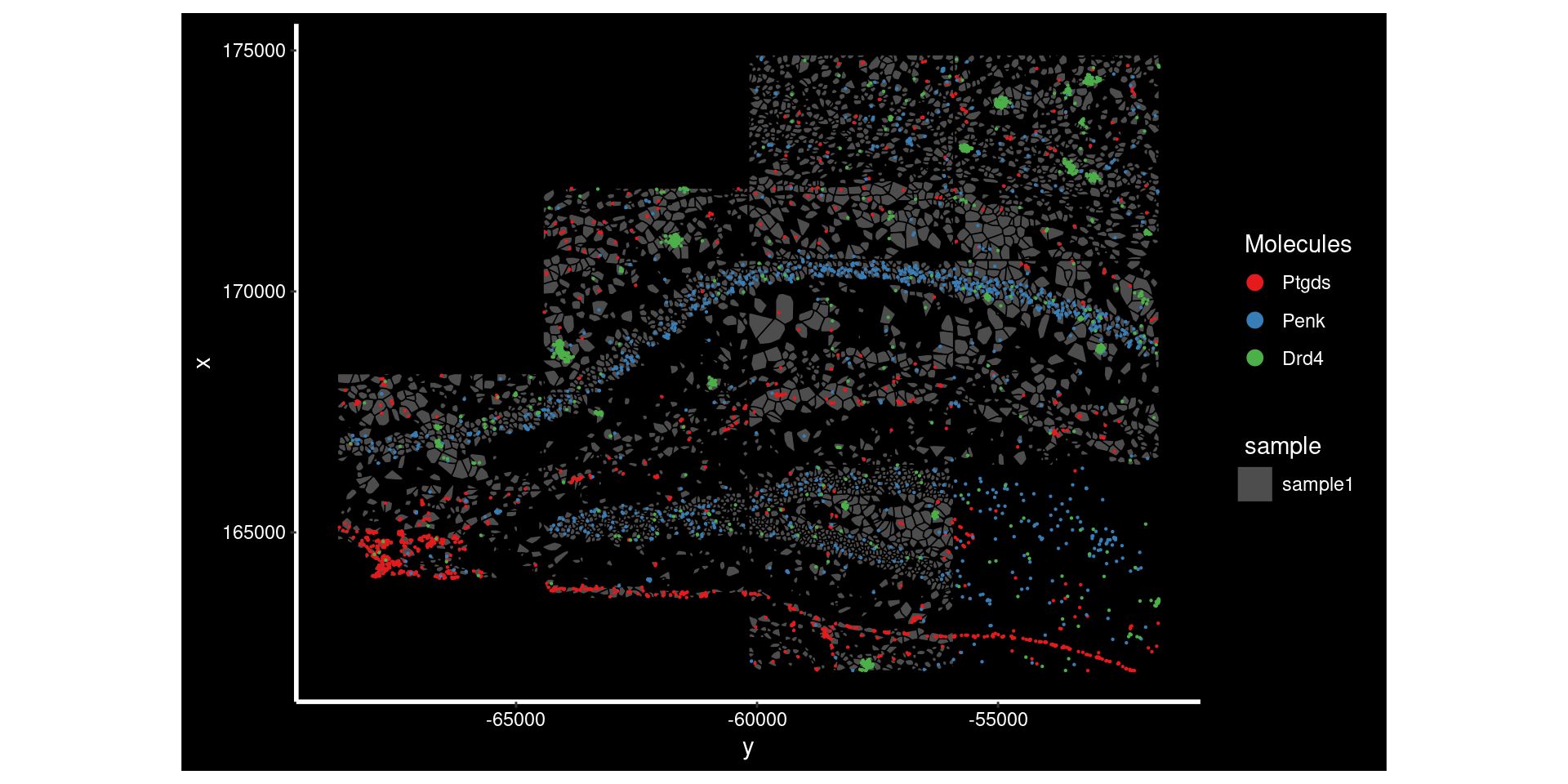

Can also show the celltypes present at those locations, though it can be hard to read.

ImageDimPlot(so.sample,  fov = "AD2.AD3.CosMx",
             molecules = top_genes, 
             group.by = 'cluster_name', 
             boundaries = "segmentation",
             border.color = 'black', axes = T, crop=TRUE)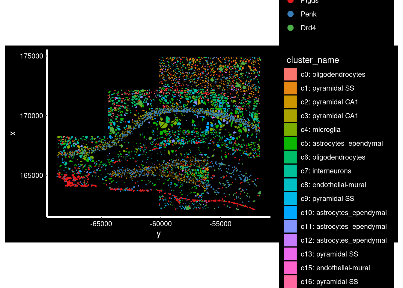

Run across all samples

We just ran that over one sample. Realistically, we would want to test multiple samples. Here we run the test on each tissue sample separately.

samples <- levels(so@meta.data$sample)
results_list <- list()

for (the_sample in samples) {
  
  so.sample <- subset( so, subset= sample == the_sample)
  
  # Again, this should be: 
  #so.sample <- FindSpatiallyVariableFeatures(
  so.sample <- FindSpatiallyVariableFeatures.Seurat_EDITED(
    so.sample, 
    assay = "RNA", 
    features = VariableFeatures(so.sample),    
    selection.method = "moransi",
    layer = "counts"
  )

  
  
  
  
  
  
  gene_metadata <- so.sample[["RNA"]]@meta.data
  results <- 
  select(gene_metadata, 
         feature, 
         MoransI_observed, 
         MoransI_p.value, 
         moransi.spatially.variable,
         moransi.spatially.variable.rank) %>% 
    filter(!is.na(moransi.spatially.variable.rank)) %>% # only tested
    arrange(moransi.spatially.variable.rank) %>%
    mutate(sample = the_sample) %>%
    select(sample, everything())

  
  results_list[[the_sample]] <- results
}

[1] ">>>> USING EDITED FUNCTION!!!! <<<"
[1] ">>>> USING EDITED FUNCTION!!!! <<<"
[1] ">>>> USING EDITED FUNCTION!!!! <<<"
[1] ">>>> USING EDITED FUNCTION!!!! <<<"

results_all <- bind_rows(results_list)

Display results for variable genes.

DT::datatable(results_all) 

Ttr had a higher MoransI score in sample4 than sample1. Plotting its distribution in both shows the difference.

ImageDimPlot(
  subset( so, subset = sample == 'sample1'),  
             fov          = "AD2.AD3.CosMx",
             molecules    = 'Ttr', 
             group.by     = 'sample', cols = c("grey30"), # Make all cells grey.
             boundaries   = "segmentation",
             border.color = 'black', axes = T, crop=TRUE)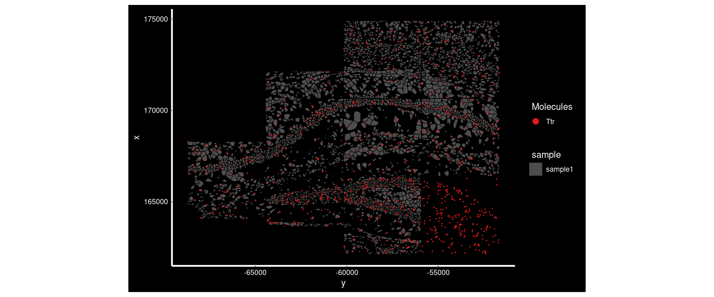

ImageDimPlot(
  subset( so, subset = sample == 'sample4'),  
             fov          = "AD4.AD5.CosMx", # note the slide it is on.
             molecules    = 'Ttr', 
             group.by     = 'sample', cols = c("grey30"), # Make all cells grey.
             boundaries   = "segmentation",
             border.color = 'black', axes = T, crop=TRUE)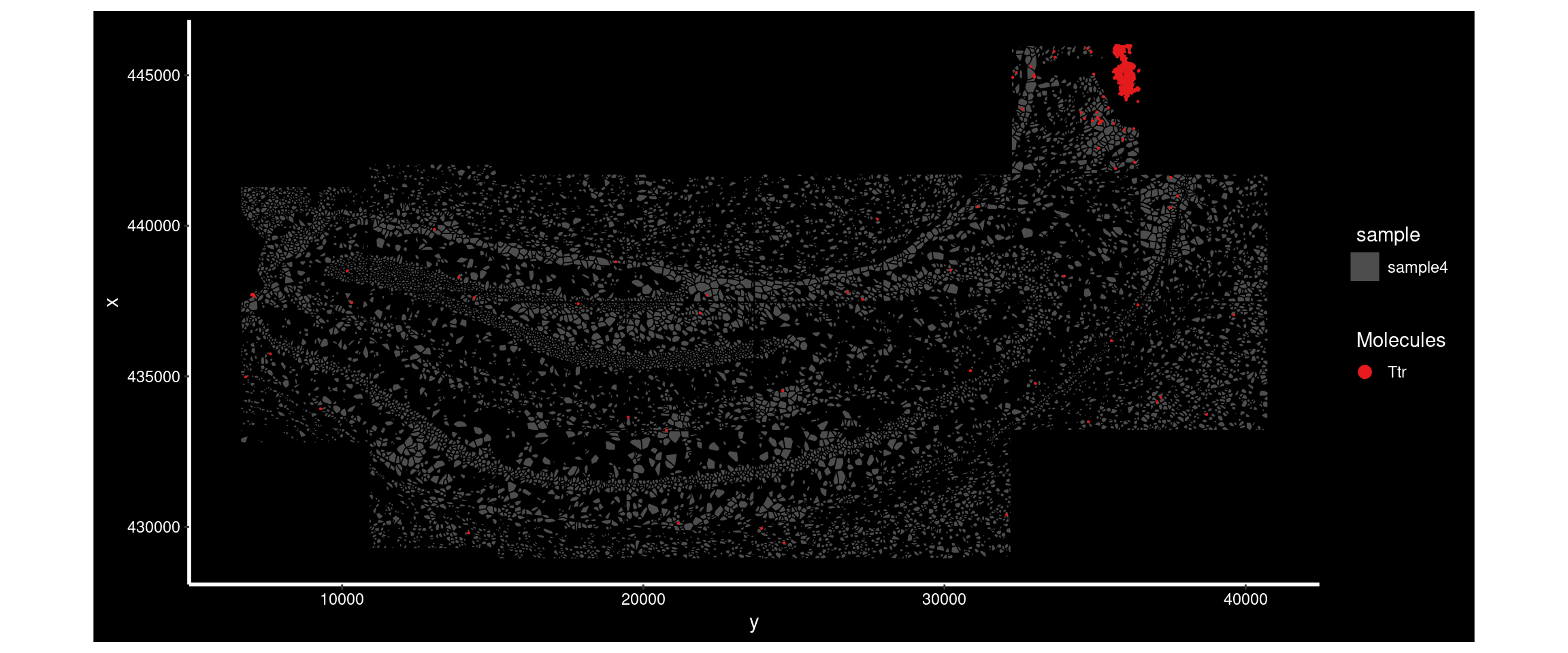

Code Snippet

Assumes that tissue samples are in a metadata column data called ‘sample’. If there are multiple slides, it may be neccessary to call joinlayers.

library(Seurat)
library(tidyverse)
library(DT)

# Load edited function, see https://github.com/satijalab/seurat/issues/8226
# Available here: https://github.com/swbioinf/spatialsnippets/blob/main/code/spatially_variable_features_code.R
source("spatially_variable_features_code.R")


# If not alread run, find variable features
num_variable_features = 1000 # Choose based on likely results and acceptable runtime
so <-  FindVariableFeatures(so, nfeatures=num_variable_features)


# Record moransI results fore ach sample one by one.
samples <- levels(so@meta.data$sample)
results_list <- list()
for (the_sample in samples) {
  
  so.sample <- subset( so, subset= sample == the_sample)
  
  # Again, this should be: 
  #so.sample <- FindSpatiallyVariableFeatures(
  so.sample <- FindSpatiallyVariableFeatures.Seurat_EDITED(
    so.sample, 
    assay = "RNA", 
    features = VariableFeatures(so.sample),    
    selection.method = "moransi",
    layer = "counts"
  )
  
  # Format output table
  gene_metadata <- so.sample[["RNA"]]@meta.data
  results <- 
  select(gene_metadata, 
         feature, 
         MoransI_observed, 
         MoransI_p.value, 
         moransi.spatially.variable,
         moransi.spatially.variable.rank) %>% 
    filter(!is.na(moransi.spatially.variable.rank)) %>% # only tested
    arrange(moransi.spatially.variable.rank) %>%
    mutate(sample = the_sample) %>%
    select(sample, everything())

  
  results_list[[the_sample]] <- results
}

# Collect output result 
results_all <- bind_rows(results_list)

Results

head(results_all)

   sample feature MoransI_observed MoransI_p.value moransi.spatially.variable
1 sample1   Ptgds       0.32296951    0.0009756098                       TRUE
2 sample1    Penk       0.15905615    0.0009756098                       TRUE
3 sample1    Drd4       0.08720462    0.0009756098                       TRUE
4 sample1  Lilra5       0.08718934    0.0009756098                       TRUE
5 sample1     Vtn       0.05282752    0.0009756098                       TRUE
6 sample1   Acta2       0.02569337    0.0009756098                       TRUE
  moransi.spatially.variable.rank
1                               1
2                               2
3                               3
4                               4
5                               5
6                               6

• feature : The gene being tested
• MoransI_observed : The moransI statistic calculated. Higher values indicate more spatial correlation, 0 is completely random, and negative values indicate anti-correlation (ie repulsion).
• MoransI_p.value : P-value for the moransI test.
• moransi.spatially.variable : Is this gene spatially restricted? True or false value.
• moransi.spatially.variable.rank : Ranking of the genes by spatial correlation, where 1 is the most distincly spatially restricted.
• sample: (not a default column, added by code): What tissue sample the test was run on.

More information

• Microglia-astrocyte crosstalk in the amyloid plaque niche of an Alzheimer’s disease mouse model, as revealed by spatial transcriptomics: Data used in this example.
• MoransI wikipedia: What is MoransI test, with pictures.
• Seurat Spatially variable features: This is actually the sequencing based technology vignette (for visium data), but it covers the FindSpatiallyVariableFeatures function
• FindSpatiallyVariableFeatures() Bug report : Link to the bug report on the Seurat repo in github. Can check the status of this issue here.
• Voyager toolkit - spatial vignette : Here is a more focussed and detailed vignette on calculating spatial statistics for gene expression using the Voyager package. It does not use Seurat objects, it is rather using the bioconductor compatible SpatialExperiment class.

References

Session information

sessionInfo()

R version 4.3.2 (2023-10-31)
Platform: x86_64-pc-linux-gnu (64-bit)
Running under: Ubuntu 22.04.5 LTS

Matrix products: default
BLAS:   /usr/lib/x86_64-linux-gnu/openblas-pthread/libblas.so.3 
LAPACK: /usr/lib/x86_64-linux-gnu/openblas-pthread/libopenblasp-r0.3.20.so;  LAPACK version 3.10.0

locale:
 [1] LC_CTYPE=en_AU.UTF-8       LC_NUMERIC=C              
 [3] LC_TIME=en_AU.UTF-8        LC_COLLATE=en_AU.UTF-8    
 [5] LC_MONETARY=en_AU.UTF-8    LC_MESSAGES=en_AU.UTF-8   
 [7] LC_PAPER=en_AU.UTF-8       LC_NAME=C                 
 [9] LC_ADDRESS=C               LC_TELEPHONE=C            
[11] LC_MEASUREMENT=en_AU.UTF-8 LC_IDENTIFICATION=C       

time zone: Etc/UTC
tzcode source: system (glibc)

attached base packages:
[1] stats     graphics  grDevices datasets  utils     methods   base     

other attached packages:
 [1] DT_0.33            lubridate_1.9.3    forcats_1.0.0      stringr_1.5.1     
 [5] dplyr_1.1.4        purrr_1.0.2        readr_2.1.5        tidyr_1.3.1       
 [9] tibble_3.2.1       ggplot2_3.5.0      tidyverse_2.0.0    Seurat_5.1.0      
[13] SeuratObject_5.0.2 sp_2.1-3           workflowr_1.7.1   

loaded via a namespace (and not attached):
  [1] RColorBrewer_1.1-3     rstudioapi_0.16.0      jsonlite_1.8.8        
  [4] magrittr_2.0.3         spatstat.utils_3.0-4   farver_2.1.1          
  [7] rmarkdown_2.26         fs_1.6.3               vctrs_0.6.5           
 [10] ROCR_1.0-11            spatstat.explore_3.2-7 htmltools_0.5.8.1     
 [13] sass_0.4.9             sctransform_0.4.1      parallelly_1.37.1     
 [16] KernSmooth_2.23-22     bslib_0.7.0            htmlwidgets_1.6.4     
 [19] ica_1.0-3              plyr_1.8.9             plotly_4.10.4         
 [22] zoo_1.8-12             cachem_1.0.8           whisker_0.4.1         
 [25] igraph_2.0.3           mime_0.12              lifecycle_1.0.4       
 [28] pkgconfig_2.0.3        Matrix_1.6-5           R6_2.5.1              
 [31] fastmap_1.1.1          fitdistrplus_1.1-11    future_1.33.2         
 [34] shiny_1.8.1.1          digest_0.6.35          colorspace_2.1-0      
 [37] patchwork_1.2.0        ps_1.7.6               rprojroot_2.0.4       
 [40] tensor_1.5             RSpectra_0.16-1        irlba_2.3.5.1         
 [43] crosstalk_1.2.1        labeling_0.4.3         RcppZiggurat_0.1.6    
 [46] progressr_0.14.0       timechange_0.3.0       fansi_1.0.6           
 [49] spatstat.sparse_3.0-3  httr_1.4.7             polyclip_1.10-6       
 [52] abind_1.4-5            compiler_4.3.2         proxy_0.4-27          
 [55] withr_3.0.0            DBI_1.2.2              fastDummies_1.7.3     
 [58] highr_0.10             MASS_7.3-60.0.1        classInt_0.4-10       
 [61] units_0.8-5            tools_4.3.2            lmtest_0.9-40         
 [64] httpuv_1.6.15          future.apply_1.11.2    Rfast2_0.1.5.2        
 [67] goftest_1.2-3          glue_1.7.0             callr_3.7.6           
 [70] nlme_3.1-164           promises_1.2.1         sf_1.0-16             
 [73] grid_4.3.2             Rtsne_0.17             getPass_0.2-4         
 [76] cluster_2.1.6          reshape2_1.4.4         generics_0.1.3        
 [79] gtable_0.3.4           spatstat.data_3.0-4    tzdb_0.4.0            
 [82] class_7.3-22           hms_1.1.3              data.table_1.15.4     
 [85] utf8_1.2.4             spatstat.geom_3.2-9    RcppAnnoy_0.0.22      
 [88] ggrepel_0.9.5          RANN_2.6.1             pillar_1.9.0          
 [91] spam_2.10-0            RcppHNSW_0.6.0         later_1.3.2           
 [94] splines_4.3.2          lattice_0.22-6         renv_1.0.5            
 [97] survival_3.5-8         deldir_2.0-4           tidyselect_1.2.1      
[100] Rnanoflann_0.0.3       miniUI_0.1.1.1         pbapply_1.7-2         
[103] knitr_1.45             git2r_0.33.0           gridExtra_2.3         
[106] scattermore_1.2        xfun_0.43              matrixStats_1.2.0     
[109] stringi_1.8.3          lazyeval_0.2.2         yaml_2.3.8            
[112] evaluate_0.23          codetools_0.2-20       BiocManager_1.30.22   
[115] cli_3.6.2              RcppParallel_5.1.7     uwot_0.1.16           
[118] xtable_1.8-4           reticulate_1.35.0      munsell_0.5.1         
[121] processx_3.8.4         jquerylib_0.1.4        Rcpp_1.0.12           
[124] globals_0.16.3         spatstat.random_3.2-3  png_0.1-8             
[127] Rfast_2.1.0            parallel_4.3.2         dotCall64_1.1-1       
[130] listenv_0.9.1          viridisLite_0.4.2      e1071_1.7-14          
[133] scales_1.3.0           ggridges_0.5.6         leiden_0.4.3.1        
[136] rlang_1.1.3            cowplot_1.1.3