scRNAseq differential expression without replicates
Sarah Williams
Last updated: 2024-09-26
Checks: 7 0
Knit directory: spatialsnippets/
This reproducible R Markdown analysis was created with workflowr (version 1.7.1). The Checks tab describes the reproducibility checks that were applied when the results were created. The Past versions tab lists the development history.
Great! Since the R Markdown file has been committed to the Git repository, you know the exact version of the code that produced these results.
Great job! The global environment was empty. Objects defined in the global environment can affect the analysis in your R Markdown file in unknown ways. For reproduciblity it’s best to always run the code in an empty environment.
The command set.seed(20231017) was run prior to running
the code in the R Markdown file. Setting a seed ensures that any results
that rely on randomness, e.g. subsampling or permutations, are
reproducible.
Great job! Recording the operating system, R version, and package versions is critical for reproducibility.
Nice! There were no cached chunks for this analysis, so you can be confident that you successfully produced the results during this run.
Great job! Using relative paths to the files within your workflowr project makes it easier to run your code on other machines.
Great! You are using Git for version control. Tracking code development and connecting the code version to the results is critical for reproducibility.
The results in this page were generated with repository version 4edfd35. See the Past versions tab to see a history of the changes made to the R Markdown and HTML files.
Note that you need to be careful to ensure that all relevant files for
the analysis have been committed to Git prior to generating the results
(you can use wflow_publish or
wflow_git_commit). workflowr only checks the R Markdown
file, but you know if there are other scripts or data files that it
depends on. Below is the status of the Git repository when the results
were generated:
Ignored files:
    Ignored:    .Rhistory
    Ignored:    .Rproj.user/
    Ignored:    analysis/e_neighbourcellchanges.nb.html
    Ignored:    analysis/glossary.nb.html
    Ignored:    renv/library/
    Ignored:    renv/staging/
Note that any generated files, e.g. HTML, png, CSS, etc., are not included in this status report because it is ok for generated content to have uncommitted changes.
These are the previous versions of the repository in which changes were
made to the R Markdown (analysis/e_DEWithoutReps.Rmd) and
HTML (docs/e_DEWithoutReps.html) files. If you’ve
configured a remote Git repository (see ?wflow_git_remote),
click on the hyperlinks in the table below to view the files as they
were in that past version.
| File | Version | Author | Date | Message |
|---|---|---|---|---|
| Rmd | 4edfd35 | swbioinf | 2024-09-26 | wflow_publish("analysis/e_DEWithoutReps.Rmd") |
| html | cd1b7ad | swbioinf | 2024-09-26 | Build site. |
| Rmd | a42f6d3 | swbioinf | 2024-09-26 | wflow_publish("analysis/e_DEWithoutReps.Rmd") |
| html | 2b1c8e2 | swbioinf | 2024-09-19 | Build site. |
| Rmd | 511594f | swbioinf | 2024-09-19 | wflow_publish("analysis/") |
| html | e7a4c12 | Sarah Williams | 2023-10-18 | Build site. |
| Rmd | 507ead4 | Sarah Williams | 2023-10-18 | wflow_publish("analysis/") |
| Rmd | 584cf73 | Sarah Williams | 2023-10-17 | adding |
| html | 584cf73 | Sarah Williams | 2023-10-17 | adding |
Overview
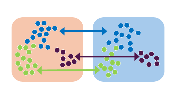
Sometimes there are no biological replicates, yet you still want to make a comparison. While not ideal, its possible. Individual cells may be treated as ‘replicates’ to explore the difference between two samples.
This requires:
- Cell clusters
- 2 or more samples (or grouping to compare)
For example:
- What genes are differentially expressed between the knockout (n=1) and control(n=1), for every cell type.
- In my n=1 pilot study - what is differentially expressed between two of my stromal clusters?
Steps:
- Filter to testable genes (enough expression to see changes)
- Test for changes in gene expression
- Plot DE results and individual genes.
Gotchas
Caveat on 1 vs 1 comparisons!
Essentially the results we get will be testing the difference between this specific sample and that specific sample. The p-values for such a test can be very significant!
But those p-values can’t be compared to those using multiple samples, and we cannot tell if our results will generalise to other samples. They are likely good candidates for further work though!
But what about pooled samples?
Note that ‘pooling’ multiple unlabelled biological samples before library prep will still count as ‘one’ replicate no many how many samples are in the pool - because we have no way to tell what sample a cell comes from. A change in gene expression could be from a single outlier sample.
NB: Using cell hashing approaches to tag samples before pooling avoids this issue.
Worked example
The data for this example is from paper Forming nephrons promote nephron progenitor maintenance and branching morphogenesis via paracrine BMP4 signalling under the control of Wnt4 (Moreau et al. 2023)
This study included 10X chromium single cell RNAseq data from 4 conditions, with 3-4 E14.5 mice pooled per group.
- Sample1 (Wnt4FloxKO): Wnt4Flox/Flox Six2-Conditional Wnt4 Knockout
- Sample2 (Wnt4FloxHet): Wnt4Flox/+ Six2-Conditional Wnt4 Het
- Sample3 (Wnt4Het): Wnt4 GCE/+ Control Wnt4 Het
- Sample4 (Wnt4KO): Wnt4 GCE/GCE Knockout Wnt4
In that paper they explain that complete or conditional homozygous knockout of Wnt4 gene results in abnormal kidney development, and they use scRNAseq data to explore effects at cellular level. (Moreau et al. 2023)
In this vignette, we will test for differential expression in each cell type for two 1 vs 1 comparisons:
- Wnt4KO vs Wnt4Het : Complete knockout vs heterozgote
- Wnt4FloxKO vs Wnt4FloxHet : Conditional (Flox) knockout vs heterozygote
Load Libraries and Data
library(Seurat)
library(edgeR)
library(limma)
library(DT)
library(tidyverse)


dataset_dir      <- '~/projects/spatialsnippets/datasets'
seurat_file      <- file.path(dataset_dir, 'Wnt4KO_Moreau2023',  "Wnt4KOE14.5_11_ss.rds")

so <- readRDS(seurat_file)
Experimental Design
In this case the sample (sample 1-4), ‘genotype’ GT effect and GT short columns are just different labels for this same groups. We will use GTshort as our ‘sample’ names throughout.
There are between 4000 and 10000 cells per sample.
select(so@meta.data, sample, Genotype, GTeffect, GTshort) %>%
  as_tibble() %>%
  group_by( sample, Genotype, GTeffect, GTshort) %>%
  summarise(num_cells=n(), .groups = 'drop') %>%
  DT::datatable()
Filter
Counts per cell
A minimum-counts-per-cell threshold was already applied to this dataset (during preprocessing) so nothing to do here.
# This is plenty
min(so$nCount_RNA)
[1] 1456Cells per group
How many cells are there for each celltype for each sample? If there are too few on either side of the contrast, we won’t be able to test.
How many is too few? 50 might be a good threshold. In this case however, we might consider being very permissive and allowing just 20 cells to look at some celltypes that are clearly reduced or increased in number between conditions (e.g. c9,c10,c11).
They’re interesting in this experiment, but have to keep in mind during interpretation that results may be less reliable.
We will apply that filter later when running the differential expression.
min_cells_per_group <- 20 # used later
table(so$CelltypeCode, so$GTshort)
                                     Wnt4FloxHet Wnt4FloxKO Wnt4Het Wnt4KO
  c0: Blood                                 1531        567    2597    189
  c1: Stroma                                 553       2014     750    130
  c2: High Mitochondria - Non Wnt4KO         868        678    1353     69
  c3: NP                                     587       1225     684    376
  c4: Stroma                                 403       1088     435    283
  c5: Stroma                                 283        587     339    511
  c6: Stroma                                 343        841     391     32
  c7: Stroma                                 326        672     242    330
  c8: Immune                                 408        701     228    144
  c9: Stroma - Wnt4KO                         33         41      23   1383
  c10: UE - Cortical                         325        408     345     35
  c11: UE - Tip                              251        466     307     47
  c12: Stroma                                189        658     177     28
  c13: Vasculature                           295        245     227     22
  c14: High Mitochondria                     125         16     140    381
  c15: Podocyte                               61         65      49    110
  c16: Blood                                 171         28       8      9
  c17: Stroma                                 21         94      13     17
  c18: Immune                                 29         59      24      6
  c19: UE - Medullary                         34         58       8      1
Run just one differential expression
Talk about options. …
- layer vs assay
- SCT vs RNA
- count vs data vs data scale
- subsampling
- min.pct
      de_result <- FindMarkers(so.this,
                               ident.1  = contrast[1],
                               ident.2  = contrast[2],
                               slot     = 'data',
                               test.use = "wilcox", # the default
                               min.pct  = 0.01,   # Note
                               max.cells.per.ident = 100 # 1000 # if you have really big clusters, set this to subsample!
                               )
Run differential expression for every cluster
We typically want to know about changes in every cluster. We can simply loop through and run them one-by-one. This can make for a lot of contrasts!
2x comparisons * 19x clusters = 38 sets of differential results The below code makes a big table of all the tests - recording which contrast was being done in which cluster.
NB: Note that the FindMarkers() function returns a table with feature names as a rowname. Rownames are expected to be unique. So while that is fine for one comparison, but when we want to put more together, we need to give it its own column. If we don’t, there’ll be gene names with ‘.1’ appended to the end!
# Set threhoehsolds
min_cells_per_group <- 20

# Calculate DE across every celltype
# Empty list to collect results
de_result_list     <- list()
de_result_sig_list <- list()

# the contrasts
# If we store them in a list we can give the nice names
contrast_list <-  list( # 'Test'      vs  'control'
                       FloxWnt4KOvsFloxHet  = c('Wnt4FloxKO',      'Wnt4FloxHet' ) ,
                       TotalWnt4KOvsHet     = c('Wnt4KO',          'Wnt4Het'     ) )

## Or you could autogenerated them
#make_contrast_name <- function(contrast_parts){ paste0(contrast_parts[1],"vs",contrast_parts[1])}
#contrast_names <- sapply(FUN=make_contrast_name, X=contrast_list)
#names(contrast_list) <- contrast_names


# note keeping all 4 samples before two contrasts. (actually does that matter for wilcox ranK sum - CHECK)

#the_celltype = 'c15: Podocyte'
#the_celltype = "c16: Blood"
#contrast_name <- 'TotalWnt4KOvsHet'

for (the_celltype in levels(so$CelltypeCode)[5:7]) {

  # Subset to one cell type.
  print(the_celltype)

  so.this <- subset(so, CelltypeCode == the_celltype)

  # count how many cells within each sample (GTshort)
  # And list which samples have more than the minimum
  cells_per_sample <- table(so.this$GTshort)
  print(cells_per_sample)
  samples_with_enough_cells <- names(cells_per_sample)[cells_per_sample > min_cells_per_group]

  # SUbset to only those samples (might be all cells, might be no cells)
  so.this <- subset(so.this, GTshort %in% samples_with_enough_cells)


  # For each listed contrast, do both sides of the contrast have enough cells?
  # This is of course much simpler if you only have one contrast!
  for (contrast_name in names(contrast_list)) {

    # from mycontrastname pull out list of the two samples involved;
    # c('test', 'control')
    contrast <- contrast_list[[contrast_name]]

    # Only run this contrast if both sides pass!
    if (all(contrast %in% samples_with_enough_cells)) {
      print(contrast_name)

      # We need to tell Seurat to group by _sample_ not cluster.
      Idents(so.this) <- so.this$GTshort


      de_result <- FindMarkers(so.this,
                               ident.1  = contrast[1],
                               ident.2 = contrast[2],
                               slot     = 'data',
                               test.use = "wilcox", # the default
                               min.pct  = 0.01,   # Note
                               max.cells.per.ident = 100 # 1000 # if you have really big clusters, set this to subsample!
                               )


      # It can be helpful to know the average expression of a gene
      # This will give us the average (per cell) within this celltype.
      avg_expression <- rowMeans(GetAssayData(so.this, assay = 'SCT', layer="data"))


      de_result.formatted <- de_result %>%
      rownames_to_column("target") %>%
      mutate(contrast=contrast_name,
             celltype=the_celltype,
             avg_expression=avg_expression[target]) %>%
      select(celltype,contrast,target,avg_expression, everything()) %>%
      arrange(p_val)

      # Filter to just significant results, optionally by log2FC.
      de_result.sig <- filter(de_result.formatted,
                         p_val_adj < 0.01,
                         abs(avg_log2FC) > log2(1.5) )

      # Record these results in a list to combine
      full_name <- paste(contrast_name, the_celltype)
      de_result_list[[full_name]] <- de_result.formatted
      de_result_sig_list[[full_name]] <- de_result.sig

    }
  }
}
[1] "c4: Stroma"
Wnt4FloxHet Wnt4FloxKO Wnt4Het Wnt4KO
403 1088 435 283
[1] "FloxWnt4KOvsFloxHet"
[1] "TotalWnt4KOvsHet"
[1] "c5: Stroma"
Wnt4FloxHet Wnt4FloxKO Wnt4Het Wnt4KO
283 587 339 511
[1] "FloxWnt4KOvsFloxHet"
[1] "TotalWnt4KOvsHet"
[1] "c6: Stroma"
Wnt4FloxHet Wnt4FloxKO Wnt4Het Wnt4KO
343 841 391 32
[1] "FloxWnt4KOvsFloxHet"
[1] "TotalWnt4KOvsHet"# Join together results for all celltypes, and pull out those with a singificant adjusted p-value
de_results_all <- bind_rows(de_result_list)
de_results_sig <- bind_rows(de_result_sig_list)Check out the full set of significant DE genes
DT::datatable(de_results_sig)Save the results.
# Save the full set of results as a tab-deliminated text file.
# This is useful for parsing later e.g. for functional enrichment
write_tsv(x = de_results_all, "~/myproject/de_results_all.tsv")

# If you don't have too many contrasts and celltypes,
# you can save it as an excel file, with each contrast in a seprate tab.
library(writexl)
write_xlsx(de_result_list,      "~/myproject/de_results_all.xlsx")
write_xlsx(de_result_sig_list,  "~/myproject/de_results_sig.xlsx")
Check individual results
Plot some example genes.
Discuss (how to pick stuff thats real)
- further filtering - where small significant changes dominate
- violin plots are hard to read
- MA style plots.
Code Snippet
Copy and paste this bit into your own script to adapt to your own data. Make as generic as possible, just a framework.
# This code does not runResults
DT::datatable(de_result.sig)- celltype: The cluster or celltype the contrat is within. Added by running code.
- contrast: The name of what is being compared. Added by running code.
- target : Gene name. (NB: Added by our running code, in the direct output of FindMarkers(), these are row names instead)
- avg_expression : Average expression of target within celltype group. (Added by running code)
- p_val : P value without multiple hypothesis correction - see p_val_adj
- avg_log2FC : Average log 2 fold change of the comparison. Is calculated as: log2(test expression) - log2(control expression) A value of 0 represents no change, +1 is a doubling, and -1 is a halving of expression.
- pct.1 : Percent of cells in group 1 (generally test) that express the gene at all.
- pct.2 : Percent of cells in group 2 (generally control/WT/reference) that express the gene at all.
- p_val_adj : Pvalue with multiple hypothesis correction. This may be used for filtering.
More information
List of useful resources. Papers, vignettes, pertinent forum posts
Wnt4 KO in developing mouse kidney - 10X Chromium scRNAseq: Forming nephrons promote nephron progenitor maintenance and branching morphogenesis via paracrine BMP4 signalling under the control of Wnt4 (Moreau et al. 2023) : The paper with this data.
Seurat Differential Expression Vignette : How to do differential expression with the seurat package. Tells you how to use the multiple statistical tests that seurat offers.
OSCA Differntial Expression: The excellent book Orchestrating single cell analysis includes a section on differential expression, it focusses on pseuboulk approaches with replicates (which can’t be used for a 1 vs 1) using the bioconductor toolkit, but provides useful background.
Refereneces
sessionInfo()R version 4.3.2 (2023-10-31)
Platform: x86_64-pc-linux-gnu (64-bit)
Running under: Ubuntu 22.04.4 LTS
Matrix products: default
BLAS: /usr/lib/x86_64-linux-gnu/openblas-pthread/libblas.so.3
LAPACK: /usr/lib/x86_64-linux-gnu/openblas-pthread/libopenblasp-r0.3.20.so; LAPACK version 3.10.0
locale:
[1] LC_CTYPE=en_AU.UTF-8 LC_NUMERIC=C
[3] LC_TIME=en_AU.UTF-8 LC_COLLATE=en_AU.UTF-8
[5] LC_MONETARY=en_AU.UTF-8 LC_MESSAGES=en_AU.UTF-8
[7] LC_PAPER=en_AU.UTF-8 LC_NAME=C
[9] LC_ADDRESS=C LC_TELEPHONE=C
[11] LC_MEASUREMENT=en_AU.UTF-8 LC_IDENTIFICATION=C
time zone: Etc/UTC
tzcode source: system (glibc)
attached base packages:
[1] stats graphics grDevices datasets utils methods base
other attached packages:
[1] lubridate_1.9.3 forcats_1.0.0 stringr_1.5.1 dplyr_1.1.4
[5] purrr_1.0.2 readr_2.1.5 tidyr_1.3.1 tibble_3.2.1
[9] ggplot2_3.5.0 tidyverse_2.0.0 DT_0.33 edgeR_4.0.16
[13] limma_3.58.1 Seurat_5.1.0 SeuratObject_5.0.2 sp_2.1-3
[17] workflowr_1.7.1
loaded via a namespace (and not attached):
[1] RColorBrewer_1.1-3 rstudioapi_0.16.0 jsonlite_1.8.8
[4] magrittr_2.0.3 spatstat.utils_3.0-4 rmarkdown_2.26
[7] fs_1.6.3 vctrs_0.6.5 ROCR_1.0-11
[10] spatstat.explore_3.2-7 htmltools_0.5.8.1 sass_0.4.9
[13] sctransform_0.4.1 parallelly_1.37.1 KernSmooth_2.23-22
[16] bslib_0.7.0 htmlwidgets_1.6.4 ica_1.0-3
[19] plyr_1.8.9 plotly_4.10.4 zoo_1.8-12
[22] cachem_1.0.8 whisker_0.4.1 igraph_2.0.3
[25] mime_0.12 lifecycle_1.0.4 pkgconfig_2.0.3
[28] Matrix_1.6-5 R6_2.5.1 fastmap_1.1.1
[31] fitdistrplus_1.1-11 future_1.33.2 shiny_1.8.1.1
[34] digest_0.6.35 colorspace_2.1-0 patchwork_1.2.0
[37] ps_1.7.6 rprojroot_2.0.4 tensor_1.5
[40] RSpectra_0.16-1 irlba_2.3.5.1 crosstalk_1.2.1
[43] progressr_0.14.0 timechange_0.3.0 fansi_1.0.6
[46] spatstat.sparse_3.0-3 httr_1.4.7 polyclip_1.10-6
[49] abind_1.4-5 compiler_4.3.2 withr_3.0.0
[52] fastDummies_1.7.3 MASS_7.3-60.0.1 tools_4.3.2
[55] lmtest_0.9-40 httpuv_1.6.15 future.apply_1.11.2
[58] goftest_1.2-3 glue_1.7.0 callr_3.7.6
[61] nlme_3.1-164 promises_1.2.1 grid_4.3.2
[64] Rtsne_0.17 getPass_0.2-4 cluster_2.1.6
[67] reshape2_1.4.4 generics_0.1.3 gtable_0.3.4
[70] spatstat.data_3.0-4 tzdb_0.4.0 hms_1.1.3
[73] data.table_1.15.4 utf8_1.2.4 spatstat.geom_3.2-9
[76] RcppAnnoy_0.0.22 ggrepel_0.9.5 RANN_2.6.1
[79] pillar_1.9.0 spam_2.10-0 RcppHNSW_0.6.0
[82] later_1.3.2 splines_4.3.2 lattice_0.22-6
[85] renv_1.0.5 survival_3.5-8 deldir_2.0-4
[88] tidyselect_1.2.1 locfit_1.5-9.9 miniUI_0.1.1.1
[91] pbapply_1.7-2 knitr_1.45 git2r_0.33.0
[94] gridExtra_2.3 scattermore_1.2 xfun_0.43
[97] statmod_1.5.0 matrixStats_1.2.0 stringi_1.8.3
[100] lazyeval_0.2.2 yaml_2.3.8 evaluate_0.23
[103] codetools_0.2-20 BiocManager_1.30.22 cli_3.6.2
[106] uwot_0.1.16 xtable_1.8-4 reticulate_1.35.0
[109] munsell_0.5.1 processx_3.8.4 jquerylib_0.1.4
[112] Rcpp_1.0.12 globals_0.16.3 spatstat.random_3.2-3
[115] png_0.1-8 parallel_4.3.2 dotCall64_1.1-1
[118] listenv_0.9.1 viridisLite_0.4.2 scales_1.3.0
[121] ggridges_0.5.6 leiden_0.4.3.1 rlang_1.1.3
[124] cowplot_1.1.3