Overview Fig: Properties of DFEs across Delta_SIFT classes
Thomas B
12/9/2020 Last update:(last update 2021-03-13)
Last updated: 2021-03-13
Checks: 7 0
Knit directory: delta-sift-polydfe/
This reproducible R Markdown analysis was created with workflowr (version 1.6.2). The Checks tab describes the reproducibility checks that were applied when the results were created. The Past versions tab lists the development history.
Great! Since the R Markdown file has been committed to the Git repository, you know the exact version of the code that produced these results.
Great job! The global environment was empty. Objects defined in the global environment can affect the analysis in your R Markdown file in unknown ways. For reproduciblity it’s best to always run the code in an empty environment.
The command set.seed(20210313) was run prior to running the code in the R Markdown file. Setting a seed ensures that any results that rely on randomness, e.g. subsampling or permutations, are reproducible.
Great job! Recording the operating system, R version, and package versions is critical for reproducibility.
Nice! There were no cached chunks for this analysis, so you can be confident that you successfully produced the results during this run.
Great job! Using relative paths to the files within your workflowr project makes it easier to run your code on other machines.
Great! You are using Git for version control. Tracking code development and connecting the code version to the results is critical for reproducibility.
The results in this page were generated with repository version 66965e5. See the Past versions tab to see a history of the changes made to the R Markdown and HTML files.
Note that you need to be careful to ensure that all relevant files for the analysis have been committed to Git prior to generating the results (you can use wflow_publish or wflow_git_commit). workflowr only checks the R Markdown file, but you know if there are other scripts or data files that it depends on. Below is the status of the Git repository when the results were generated:
Ignored files:
    Ignored:    .DS_Store

Untracked files:
    Untracked:  data/summary_polyDFE_siftCate_new.txt
    Untracked:  eps_vs_delta.pdf
    Untracked:  eps_vs_lognsyn_counts.pdf
    Untracked:  flux_benef_vsdelta.pdf
    Untracked:  overview_dfe_bins_ByDelta.pdf
    Untracked:  pb_versus_delta.pdf
    Untracked:  pin_pis_corrected_vs_delta.png

Unstaged changes:
    Deleted:    analysis/S1_Stat_models_deltaDIFT_DFEs.Rmd
Note that any generated files, e.g. HTML, png, CSS, etc., are not included in this status report because it is ok for generated content to have uncommitted changes.
These are the previous versions of the repository in which changes were made to the R Markdown (analysis/S2_Summary_Figure_deltaSIFT_DFEs.Rmd) and HTML (docs/S2_Summary_Figure_deltaSIFT_DFEs.html) files. If you’ve configured a remote Git repository (see ?wflow_git_remote), click on the hyperlinks in the table below to view the files as they were in that past version.
| File | Version | Author | Date | Message |
|---|---|---|---|---|
| Rmd | 6ef954c | Thomas Bataillon | 2021-03-13 | wflow_git_commit(files = "analysis/*.Rmd") |
brief overview of analysis and updates :
We read in the data made available in the lastest version of the poyDFE outputs summary by Jun Chen.
We define a covariate \(\delta\) as the change in discretized SIFT scores
We filter away the cases where eps is too big
Rationale for conditioning DFE on \(\delta\) is to illustrate that change in SIFT scores are a powerful way to capture the expected effect of mutations and the fact that DFEs are quite different. There is a sharp divide between \(\delta \leq 0\) and \(\delta >0\)
Reading the data
Note by TB Jan 14. Original analysis is made using the output summaries stored in Data/20201207/summary_PolyDFEOut.txt. Here I updated
dfe_sift <- read.table("Data/summary_polyDFE_siftCate_new.txt",header=T)

dim(dfe_sift)
[1] 507 26names(dfe_sift) [1] "species" "group" "category" "cat04" "from"
[6] "to" "mutation" "gradient" "eps" "Sd"
[11] "beta" "pb" "Sb" "alpha" "PiS"
[16] "PiN" "PiNPiS" "syn_counts" "nsyn_counts" "Lsyn"
[21] "Lnsyn" "D1" "D2" "D3" "D4"
[26] "D5" dfe_sift$delta <- dfe_sift$to - dfe_sift$fromTechnical check: distribution of \(\epsilon_{anc}\)
It looks like a few species have a really worrying estimated error epsilon_anc rate of SNP orientation and I think that all inference with eps> 0.2 should hardly be trusted ..
qplot(log10(dfe_sift$eps), bins=20) + xlab("rate of SNP polarization error (eps_anc)")+theme_minimal(base_size = 16)Warning: Removed 6 rows containing non-finite values (stat_bin).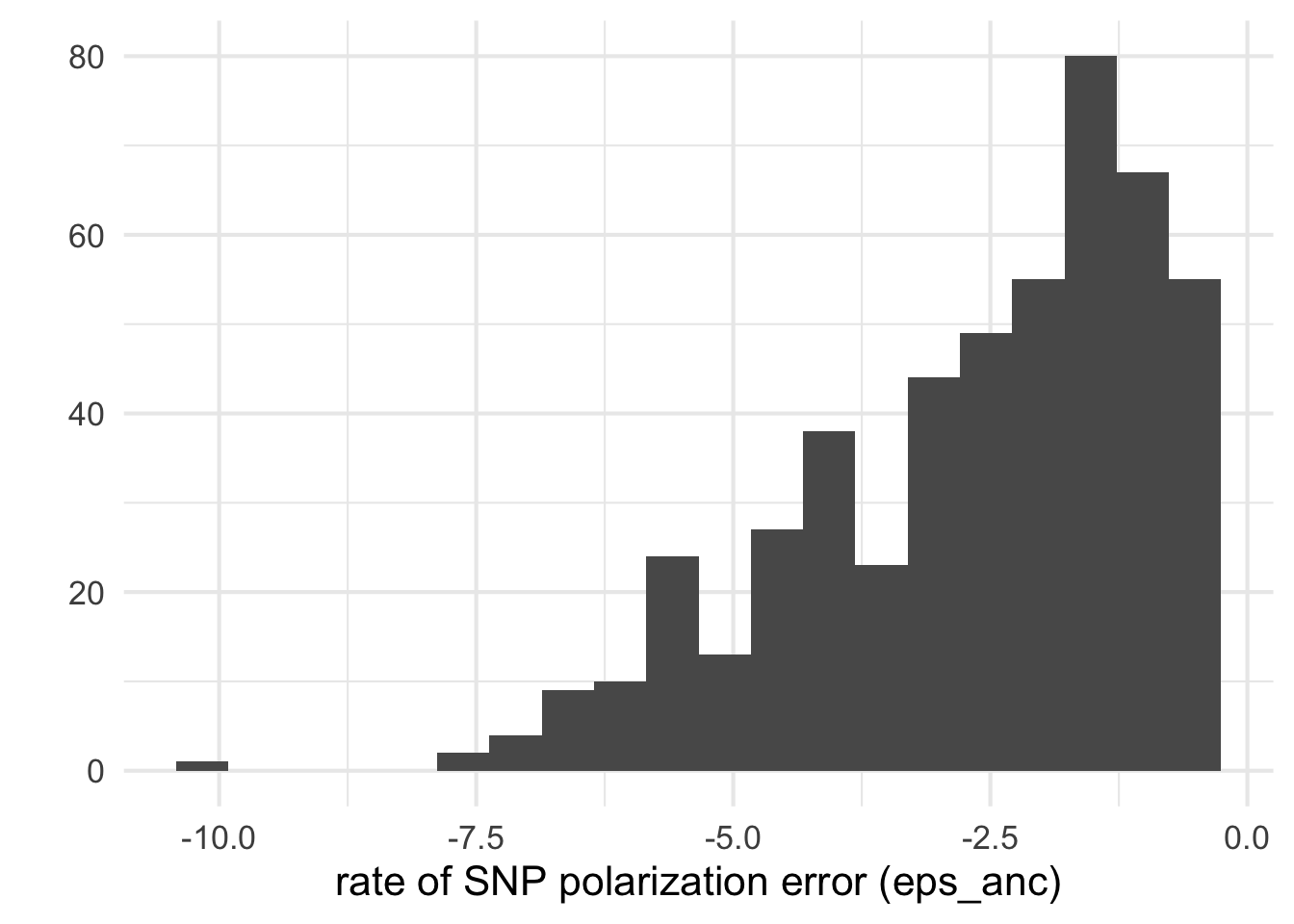
names(dfe_sift) [1] "species" "group" "category" "cat04" "from"
[6] "to" "mutation" "gradient" "eps" "Sd"
[11] "beta" "pb" "Sb" "alpha" "PiS"
[16] "PiN" "PiNPiS" "syn_counts" "nsyn_counts" "Lsyn"
[21] "Lnsyn" "D1" "D2" "D3" "D4"
[26] "D5" "delta" dfe_sift %>%
filter(nsyn_counts>100) %>%
ggplot(aes(x= log10(nsyn_counts),
y = log10(eps+0.000001),
weight=sqrt(1+nsyn_counts))) +
geom_point(aes(color = (delta<=0)), size=0.5) +
# geom_abline(intercept = log10(0.1), slope=0, color ="cornflowerblue")+
geom_smooth(method="loess", color= "cornflowerblue", span=0.5, se=T)+
ylab("rate of SNP polarization error, log10(eps)")+
xlab("SFS sample size, log10( non-syn. counts in SFS)")+
scale_color_colorblind()+
theme_cowplot(font_size = 16)+
theme(legend.position = c(0.8,0.2))+
theme(legend.background = element_rect("grey"))+
ggsave2(filename = "eps_vs_lognsyn_counts.pdf", device = "pdf")+
NULLSaving 7 x 5 in image`geom_smooth()` using formula 'y ~ x'
`geom_smooth()` using formula 'y ~ x'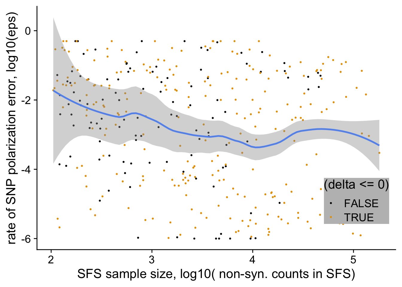
dfe_sift %>%
  filter(nsyn_counts>100) %>%
  ggplot(aes(x=delta, y = log10(eps + 0.000001), color=species, size = sqrt(nsyn_counts), weight=sqrt(1+nsyn_counts) ))+
  geom_jitter(height = 0,width = 0.1)+
  geom_smooth(method = "loess", aes(color = NULL), color = "black", span=0.75)+
  # geom_smooth(method = "lm", aes(color = NULL), color = "black", se =T)+
  theme_cowplot(font_size  = 13)+
  # facet_wrap(~group)+
  scale_color_viridis_d()+
  theme(legend.position = "none")+
  xlab(expression(delta))+
  ylab("rate of SNP polarization error, log10(eps)")+
  scale_size("counts in n-syn SFS", range=c(1,4))+
  ggsave2(filename = "eps_vs_delta.pdf", device = "pdf")+
  NULL
Saving 7 x 5 in image`geom_smooth()` using formula 'y ~ x'
`geom_smooth()` using formula 'y ~ x'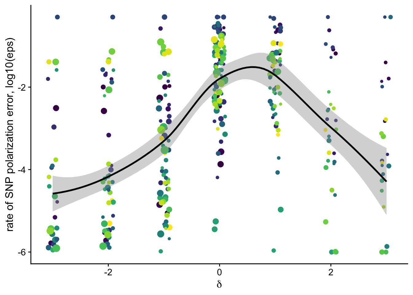
Filtering data before figure
We exclude:
* the \(\epsilon_{anc}\) > 0.1 * the number of chromosomes in the sfs < 6 species_low_nchr(manually curated list below)
unique(dfe_sift$species) [1] "Ayon" "Alyr" "Atha" "Bnana" "Bpend" "Cgrand"
[7] "Cjap" "Cmag" "Crubel" "Gprzew" "Dsin" "Lform"
[13] "Zmays" "Peuph" "Pilcif" "Pnigra" "Pruni" "Ptrich"
[19] "Qacut" "Qdent" "Lacaly" "Qmango" "Qvaria" "Sbicolor"
[25] "Shab" "Shua" "Ddyer" species_low_nchr <- c("Qmango", "Shua", "Bnana")
dfe_sift <- dfe_sift %>%
filter(!(species %in% species_low_nchr)) %>%
filter(eps <0.1) #
dim(dfe_sift)[1] 387 27The Flux of beneficial mutations \(p_b s_b\)
Detecting beneficial mutations is notoriously difficult as they are expected to be overall quite rare and therefore make a modest contribution to SFS counts. But \(\delta\) is a very relevant covariate Among the classes of mutations categorized as likely deleterious (negative \(\delta\)) we have virtually zero flux of beneficial mutations; but as \(\delta\) increases, so does the flux of beneficial mutations \(p_b S_b\):
the Flux \(p_b*S_b\)
Sylvain: The same but in log-scale
dfe_sift %>%
  filter(cat04==0) %>%
  ggplot(aes(x=delta, y=pb*Sb, color=species, weight = sqrt(1+nsyn_counts))) +
  # geom_point(aes(size = nsyn_counts))+
  geom_jitter(height = 0,width = 0.1, aes(size = sqrt(1+nsyn_counts)))+
  scale_y_log10() +
  # facet_wrap(~ group) +
  geom_smooth(method = "loess", formula ="y~ x", se =T, aes(color = NULL), color = "black", span=0.65)+
  theme_minimal(base_size = 15)+
  xlab(expression(delta))+
  ylab("Flux of beneficial mutation: pb*Sb")+
  scale_color_viridis_d()+
  theme(legend.position = "none")+
  ggsave2(filename = "flux_benef_vsdelta.pdf", device = "pdf")+
  NULL
Saving 7 x 5 in image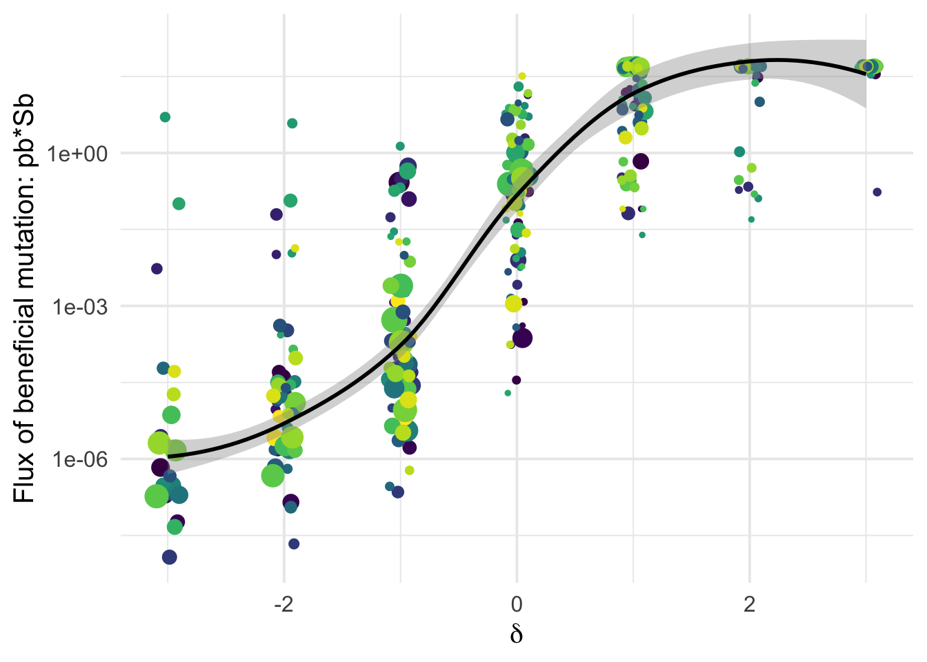
the mere proportion \(p_b\)
Sylvain: The same but in log-scale
dfe_sift %>%
  filter(cat04==0) %>%
  ggplot(aes(x=delta, y=pb, color=species, weight = 1+nsyn_counts)) +
  # geom_point(aes(size = nsyn_counts))+
  geom_jitter(height = 0, width = 0.1, aes(size = sqrt(1+nsyn_counts)))+
  # facet_wrap(~ group) +
  geom_smooth(method = "loess", formula = y ~ x, se =T, aes(color = NULL), color = "black", span=0.7 )+
  theme_minimal(base_size = 15)+
  xlab(expression(delta))+
  ylab("proportion of beneficial mutations")+
  scale_color_viridis_d()+
  theme(legend.position = "none")+
  ggsave2(filename = "pb_versus_delta.pdf",device = "pdf")+
  NULL
Saving 7 x 5 in image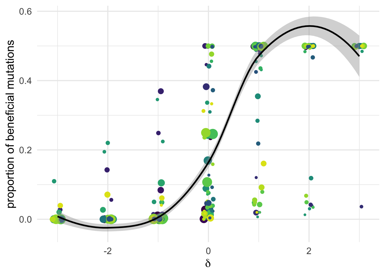
Binning of DFE by \(N_e s\)
Poportion of mutations in Nes classes
We can see that conditioning on the \(\delta\) covariates is very informative: there is a strong covariation between the proportion of mutations in Ne*s classes inferred via polyDFE and the perceived functional categories as obtained via SIFT:
dfe_sift %>%
  filter(cat04==0) %>%
  ggplot(aes(x=delta, y= D1,  weight= 1+nsyn_counts)) +
  geom_point(aes(size = nsyn_counts, color=species ))+
  # facet_wrap(~ group) +
  geom_smooth(method = "loess", formula ="y~ x", se =T, span = 0.5)+
  theme_minimal(base_size = 15)+
  xlab(expression(delta))+
  ylab("prop in Nes[0-1]")+
  scale_color_viridis_d()+
  theme(legend.position = "none")+
  NULL
Warning in simpleLoess(y, x, w, span, degree = degree, parametric =
parametric, : pseudoinverse used at -1Warning in simpleLoess(y, x, w, span, degree = degree, parametric =
parametric, : neighborhood radius 1Warning in simpleLoess(y, x, w, span, degree = degree, parametric =
parametric, : reciprocal condition number 0Warning in simpleLoess(y, x, w, span, degree = degree, parametric =
parametric, : There are other near singularities as well. 1Warning in predLoess(object$y, object$x, newx = if
(is.null(newdata)) object$x else if (is.data.frame(newdata))
as.matrix(model.frame(delete.response(terms(object)), : pseudoinverse used at -1Warning in predLoess(object$y, object$x, newx = if
(is.null(newdata)) object$x else if (is.data.frame(newdata))
as.matrix(model.frame(delete.response(terms(object)), : neighborhood radius 1Warning in predLoess(object$y, object$x, newx = if
(is.null(newdata)) object$x else if (is.data.frame(newdata))
as.matrix(model.frame(delete.response(terms(object)), : reciprocal condition
number 0Warning in predLoess(object$y, object$x, newx = if
(is.null(newdata)) object$x else if (is.data.frame(newdata))
as.matrix(model.frame(delete.response(terms(object)), : There are other near
singularities as well. 1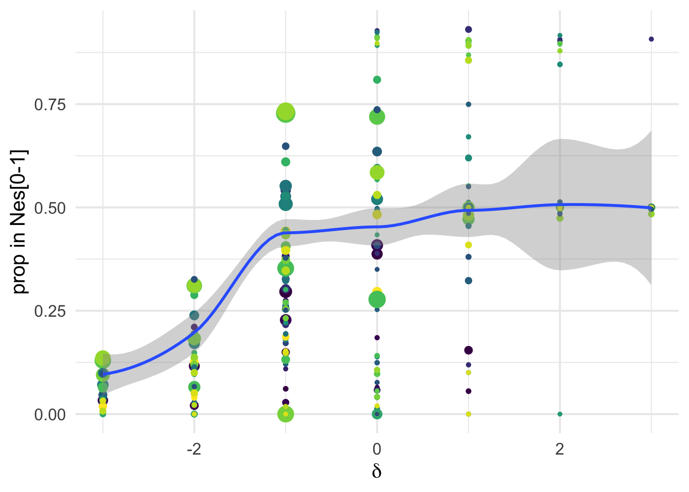
dfe_sift %>%
  filter(cat04==0) %>%
  ggplot(aes(x=delta, y= D2,  weight= 1+nsyn_counts)) +
  geom_point(aes(size = nsyn_counts, color=species))+
  # facet_wrap(~ group) +
  geom_smooth(method = "loess", formula ="y~ x", se =T, span =.5)+
  theme_minimal(base_size = 15)+
  xlab(expression(delta))+
  ylab("prop in Nes[-1, -10]")+
  scale_color_viridis_d()+
  theme(legend.position = "none")+
  NULL
Warning in simpleLoess(y, x, w, span, degree = degree, parametric =
parametric, : pseudoinverse used at -1Warning in simpleLoess(y, x, w, span, degree = degree, parametric =
parametric, : neighborhood radius 1Warning in simpleLoess(y, x, w, span, degree = degree, parametric =
parametric, : reciprocal condition number 0Warning in simpleLoess(y, x, w, span, degree = degree, parametric =
parametric, : There are other near singularities as well. 1Warning in predLoess(object$y, object$x, newx = if
(is.null(newdata)) object$x else if (is.data.frame(newdata))
as.matrix(model.frame(delete.response(terms(object)), : pseudoinverse used at -1Warning in predLoess(object$y, object$x, newx = if
(is.null(newdata)) object$x else if (is.data.frame(newdata))
as.matrix(model.frame(delete.response(terms(object)), : neighborhood radius 1Warning in predLoess(object$y, object$x, newx = if
(is.null(newdata)) object$x else if (is.data.frame(newdata))
as.matrix(model.frame(delete.response(terms(object)), : reciprocal condition
number 0Warning in predLoess(object$y, object$x, newx = if
(is.null(newdata)) object$x else if (is.data.frame(newdata))
as.matrix(model.frame(delete.response(terms(object)), : There are other near
singularities as well. 1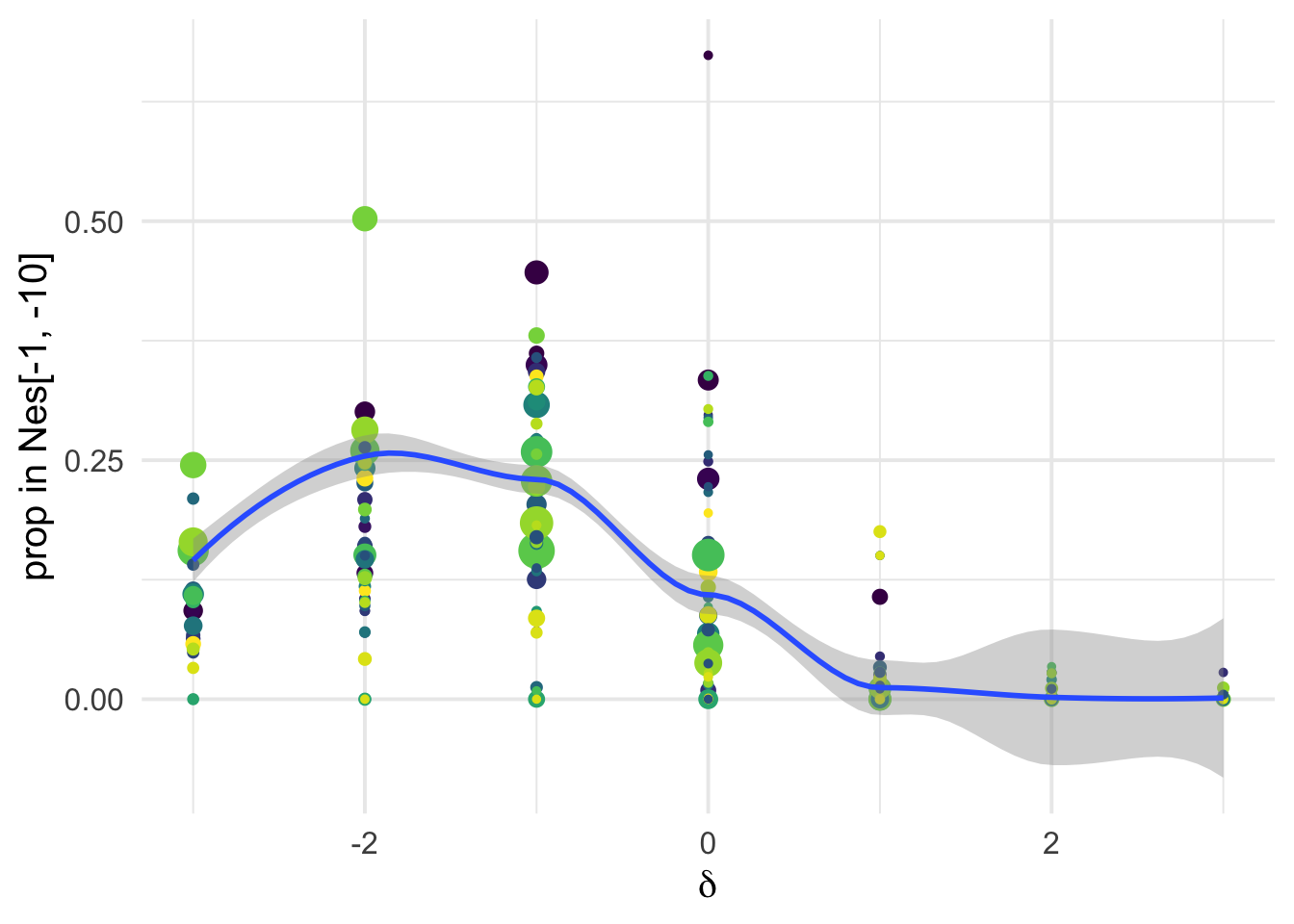
dfe_sift %>%
  filter(cat04==0) %>%
  ggplot(aes(x=delta, y= D3,  weight= 1+nsyn_counts)) +
  geom_point(aes(size = nsyn_counts, color=species))+
  # facet_wrap(~ group) +
  geom_smooth(method = "loess", formula ="y~ x", se =T)+
  theme_minimal(base_size = 15)+
  xlab(expression(delta))+
  ylab("prop in Nes[-10, -100]")+
  scale_color_viridis_d()+
  theme(legend.position = "none")+
  NULL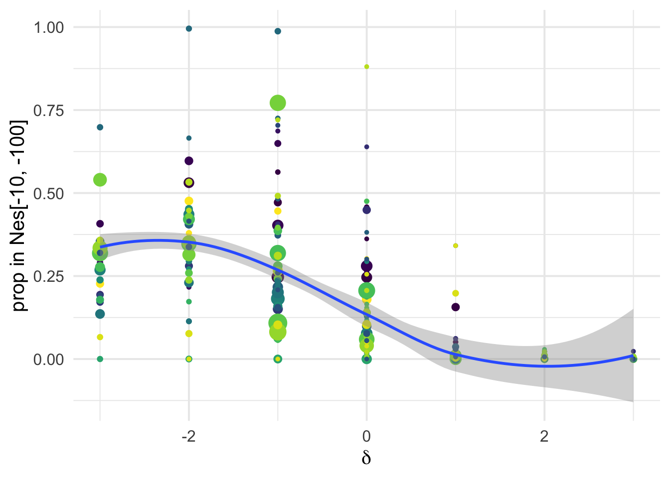
dfe_sift %>%
  filter(cat04==0) %>%
  ggplot(aes(x=delta, y= D4+D5,  weight= 1+nsyn_counts)) +
  geom_point(aes(size = nsyn_counts, color=species))+
  # facet_wrap(~ group) +
  geom_smooth(method = "loess", formula ="y~ x", se =T, span =0.5)+
  theme_minimal(base_size = 15)+
  xlab(expression(delta))+
  ylab("prop in Nes[- 100 -...]")+
  scale_color_viridis_d()+
  theme(legend.position = "none")+
  NULL
Warning in simpleLoess(y, x, w, span, degree = degree, parametric =
parametric, : pseudoinverse used at -1Warning in simpleLoess(y, x, w, span, degree = degree, parametric =
parametric, : neighborhood radius 1Warning in simpleLoess(y, x, w, span, degree = degree, parametric =
parametric, : reciprocal condition number 0Warning in simpleLoess(y, x, w, span, degree = degree, parametric =
parametric, : There are other near singularities as well. 1Warning in predLoess(object$y, object$x, newx = if
(is.null(newdata)) object$x else if (is.data.frame(newdata))
as.matrix(model.frame(delete.response(terms(object)), : pseudoinverse used at -1Warning in predLoess(object$y, object$x, newx = if
(is.null(newdata)) object$x else if (is.data.frame(newdata))
as.matrix(model.frame(delete.response(terms(object)), : neighborhood radius 1Warning in predLoess(object$y, object$x, newx = if
(is.null(newdata)) object$x else if (is.data.frame(newdata))
as.matrix(model.frame(delete.response(terms(object)), : reciprocal condition
number 0Warning in predLoess(object$y, object$x, newx = if
(is.null(newdata)) object$x else if (is.data.frame(newdata))
as.matrix(model.frame(delete.response(terms(object)), : There are other near
singularities as well. 1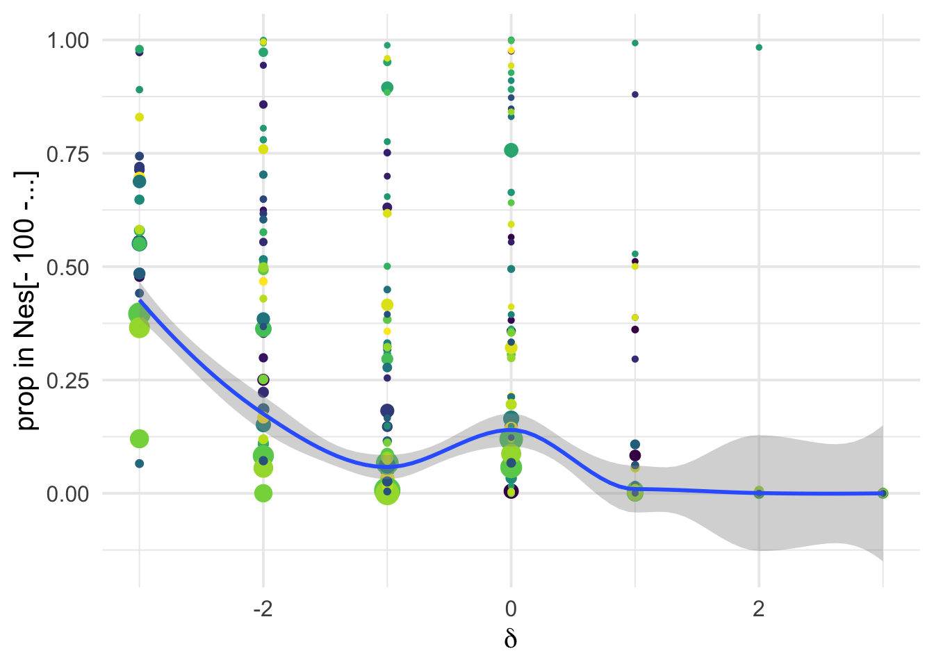
Overall figure combining
Fig Legend, each line denotes the proportion of mutations in the DFE that are beneficial (orange) or that are (increasingly) deleterious mutations : D1 ( Nes in 0-1) in light grey, D2 (Nes in 1-10) dark grey, D3(10-100 blue), D4+D5(Nes > 100) red.
 fig_overview <- dfe_sift %>%
  filter(cat04==0) %>%
  ggplot(aes(weight= 1+nsyn_counts)) +
  # geom_point(aes(size = nsyn_counts, color=species ))+
  # facet_wrap(~ group) +
   geom_smooth(aes(x=delta, y= D1),  method = "loess", formula ="y~ x", se =F, color="grey90", span = 0.5)+
  geom_smooth(aes(x=delta, y= D2),  method = "loess", formula ="y~ x", se =F, color = "grey70", span = 0.5)+
  # geom_smooth(aes(x=delta, y= D3),  method = "loess", formula ="y~ x", se =F, color = "cornflowerblue", span = 0.5)+
  geom_smooth(aes(x=delta, y= D3 +D4+D5),  method = "loess", formula ="y~ x", se =F, color = "red", span = 0.5)+
  geom_smooth(aes(x=delta, y= pb),  method = "loess", formula ="y~ x", se =F, color = "orange", span = 0.5)+
  theme_minimal(base_size = 15)+
  xlab(expression(delta))+
  ylab("prop in Nes class")+
  scale_color_viridis_d()+
  theme(legend.position = "none")+
  NULL
plot(fig_overview)
Warning in simpleLoess(y, x, w, span, degree = degree, parametric =
parametric, : pseudoinverse used at -1Warning in simpleLoess(y, x, w, span, degree = degree, parametric =
parametric, : neighborhood radius 1Warning in simpleLoess(y, x, w, span, degree = degree, parametric =
parametric, : reciprocal condition number 0Warning in simpleLoess(y, x, w, span, degree = degree, parametric =
parametric, : There are other near singularities as well. 1Warning in simpleLoess(y, x, w, span, degree = degree, parametric =
parametric, : pseudoinverse used at -1Warning in simpleLoess(y, x, w, span, degree = degree, parametric =
parametric, : neighborhood radius 1Warning in simpleLoess(y, x, w, span, degree = degree, parametric =
parametric, : reciprocal condition number 0Warning in simpleLoess(y, x, w, span, degree = degree, parametric =
parametric, : There are other near singularities as well. 1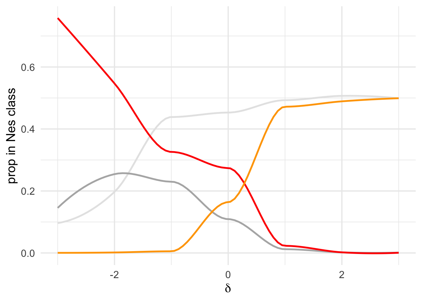
ggsave(plot = fig_overview, filename = "overview_dfe_bins_ByDelta.pdf", "pdf")Saving 7 x 5 in imageWarning in simpleLoess(y, x, w, span, degree = degree, parametric =
parametric, : pseudoinverse used at -1Warning in simpleLoess(y, x, w, span, degree = degree, parametric =
parametric, : neighborhood radius 1Warning in simpleLoess(y, x, w, span, degree = degree, parametric =
parametric, : reciprocal condition number 0Warning in simpleLoess(y, x, w, span, degree = degree, parametric =
parametric, : There are other near singularities as well. 1Warning in simpleLoess(y, x, w, span, degree = degree, parametric =
parametric, : pseudoinverse used at -1Warning in simpleLoess(y, x, w, span, degree = degree, parametric =
parametric, : neighborhood radius 1Warning in simpleLoess(y, x, w, span, degree = degree, parametric =
parametric, : reciprocal condition number 0Warning in simpleLoess(y, x, w, span, degree = degree, parametric =
parametric, : There are other near singularities as well. 1PiN/PiS corrected
Another representation by adding +1 to every count: \(\pi_N =\frac{n_N + 1}{L_N + 1}\) and \(\pi_S =\frac{n_S + 1}{L_S + 1}\) we can then directly use a log scale
dfe_sift$PiNPiScor <- (dfe_sift$nsyn_counts+1)*(dfe_sift$Lsyn+1)/((dfe_sift$Lnsyn+1)*(dfe_sift$syn_counts+1))

dfe_sift %>%
  filter(cat04==0) %>%
  ggplot(aes(x=delta, y=PiNPiScor, color=species, weight=(1+nsyn_counts)) )+
  # geom_point(aes(size = nsyn_counts)) +
  geom_jitter(width = 0.1, aes(size = nsyn_counts)) +
  scale_y_log10() +
  # facet_wrap(~ group) +
    geom_smooth(method = "loess", formula = y ~ x, se =T, aes(color = NULL), color = "black", span=0.5 )+
  # geom_smooth(method = "loess", formula ="y~ x", se =T)+
  theme_cowplot(font_size =  15)+
  xlab("Delta SIFT score")+
  ylab("corrected piN/piS")+
  scale_color_viridis_d()+
  theme(legend.position = "none")+
  ggsave2("pin_pis_corrected_vs_delta.png", device = "png")+
  NULL
Saving 7 x 5 in imageWarning in simpleLoess(y, x, w, span, degree = degree, parametric =
parametric, : pseudoinverse used at -1Warning in simpleLoess(y, x, w, span, degree = degree, parametric =
parametric, : neighborhood radius 1Warning in simpleLoess(y, x, w, span, degree = degree, parametric =
parametric, : reciprocal condition number 0Warning in simpleLoess(y, x, w, span, degree = degree, parametric =
parametric, : There are other near singularities as well. 1Warning in predLoess(object$y, object$x, newx = if
(is.null(newdata)) object$x else if (is.data.frame(newdata))
as.matrix(model.frame(delete.response(terms(object)), : pseudoinverse used at -1Warning in predLoess(object$y, object$x, newx = if
(is.null(newdata)) object$x else if (is.data.frame(newdata))
as.matrix(model.frame(delete.response(terms(object)), : neighborhood radius 1Warning in predLoess(object$y, object$x, newx = if
(is.null(newdata)) object$x else if (is.data.frame(newdata))
as.matrix(model.frame(delete.response(terms(object)), : reciprocal condition
number 0Warning in predLoess(object$y, object$x, newx = if
(is.null(newdata)) object$x else if (is.data.frame(newdata))
as.matrix(model.frame(delete.response(terms(object)), : There are other near
singularities as well. 1Warning in simpleLoess(y, x, w, span, degree = degree, parametric =
parametric, : pseudoinverse used at -1Warning in simpleLoess(y, x, w, span, degree = degree, parametric =
parametric, : neighborhood radius 1Warning in simpleLoess(y, x, w, span, degree = degree, parametric =
parametric, : reciprocal condition number 0Warning in simpleLoess(y, x, w, span, degree = degree, parametric =
parametric, : There are other near singularities as well. 1Warning in predLoess(object$y, object$x, newx = if
(is.null(newdata)) object$x else if (is.data.frame(newdata))
as.matrix(model.frame(delete.response(terms(object)), : pseudoinverse used at -1Warning in predLoess(object$y, object$x, newx = if
(is.null(newdata)) object$x else if (is.data.frame(newdata))
as.matrix(model.frame(delete.response(terms(object)), : neighborhood radius 1Warning in predLoess(object$y, object$x, newx = if
(is.null(newdata)) object$x else if (is.data.frame(newdata))
as.matrix(model.frame(delete.response(terms(object)), : reciprocal condition
number 0Warning in predLoess(object$y, object$x, newx = if
(is.null(newdata)) object$x else if (is.data.frame(newdata))
as.matrix(model.frame(delete.response(terms(object)), : There are other near
singularities as well. 1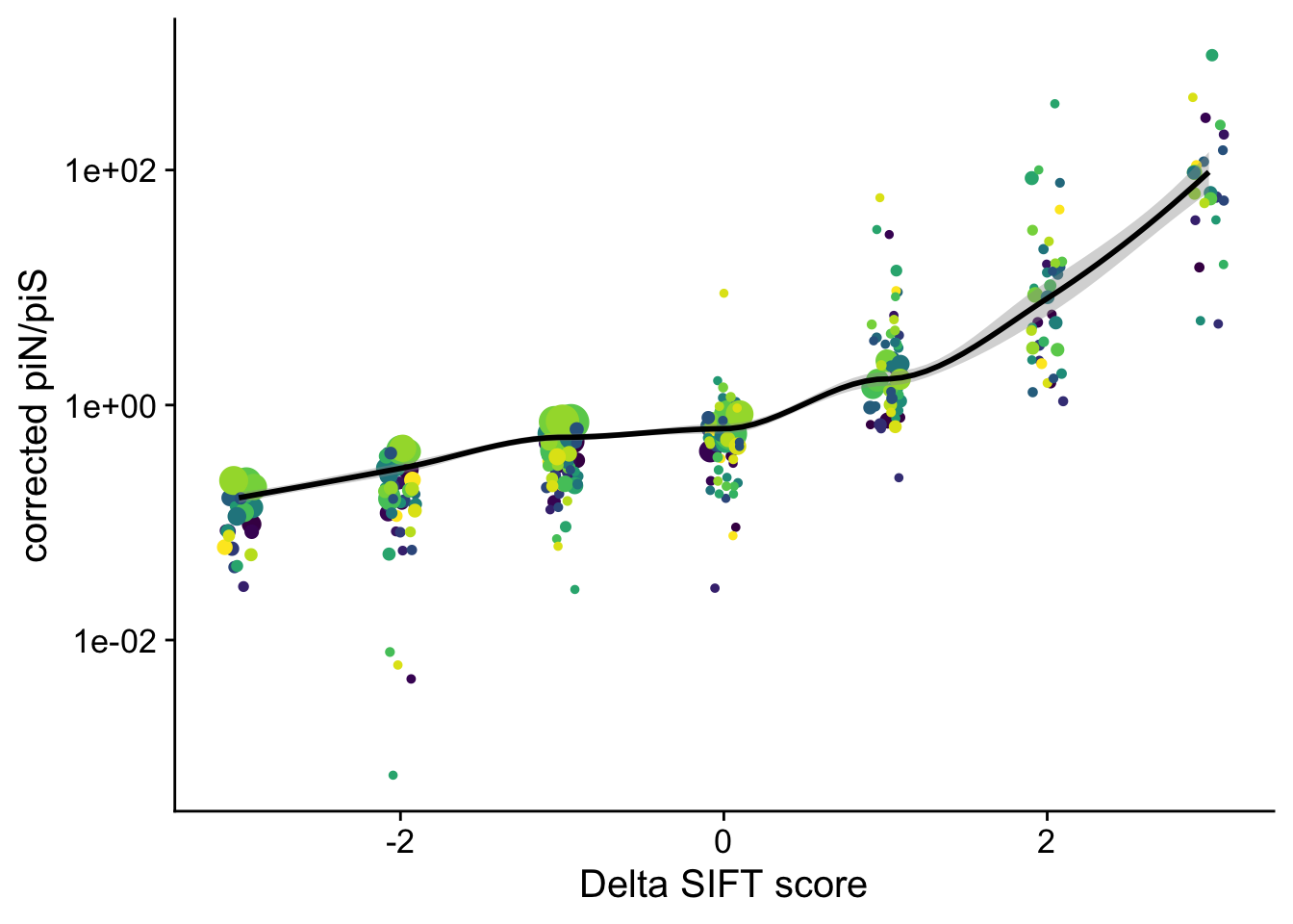
sessionInfo()R version 4.0.2 (2020-06-22)
Platform: x86_64-apple-darwin17.0 (64-bit)
Running under: macOS Catalina 10.15.7
Matrix products: default
BLAS: /Library/Frameworks/R.framework/Versions/4.0/Resources/lib/libRblas.dylib
LAPACK: /Library/Frameworks/R.framework/Versions/4.0/Resources/lib/libRlapack.dylib
locale:
[1] en_US.UTF-8/en_US.UTF-8/en_US.UTF-8/C/en_US.UTF-8/en_US.UTF-8
attached base packages:
[1] stats graphics grDevices utils datasets methods base
other attached packages:
[1] knitr_1.30 cowplot_1.1.0 magrittr_1.5 dplyr_1.0.2
[5] ggthemes_4.2.0 ggplot2_3.3.2 workflowr_1.6.2
loaded via a namespace (and not attached):
[1] Rcpp_1.0.5 pillar_1.4.6 compiler_4.0.2 later_1.1.0.1
[5] git2r_0.27.1 tools_4.0.2 digest_0.6.25 viridisLite_0.3.0
[9] lattice_0.20-41 nlme_3.1-148 evaluate_0.14 lifecycle_0.2.0
[13] tibble_3.0.3 gtable_0.3.0 mgcv_1.8-31 pkgconfig_2.0.3
[17] rlang_0.4.7 Matrix_1.2-18 rstudioapi_0.11 yaml_2.2.1
[21] xfun_0.19 withr_2.2.0 stringr_1.4.0 generics_0.0.2
[25] fs_1.5.0 vctrs_0.3.2 tidyselect_1.1.0 rprojroot_1.3-2
[29] grid_4.0.2 glue_1.4.1 R6_2.4.1 rmarkdown_2.3
[33] farver_2.0.3 purrr_0.3.4 whisker_0.4 splines_4.0.2
[37] backports_1.1.8 scales_1.1.1 promises_1.1.1 ellipsis_0.3.1
[41] htmltools_0.5.0 colorspace_1.4-1 httpuv_1.5.4 labeling_0.3
[45] stringi_1.4.6 munsell_0.5.0 crayon_1.3.4